B-spline and Bézier Geometry in OCCT

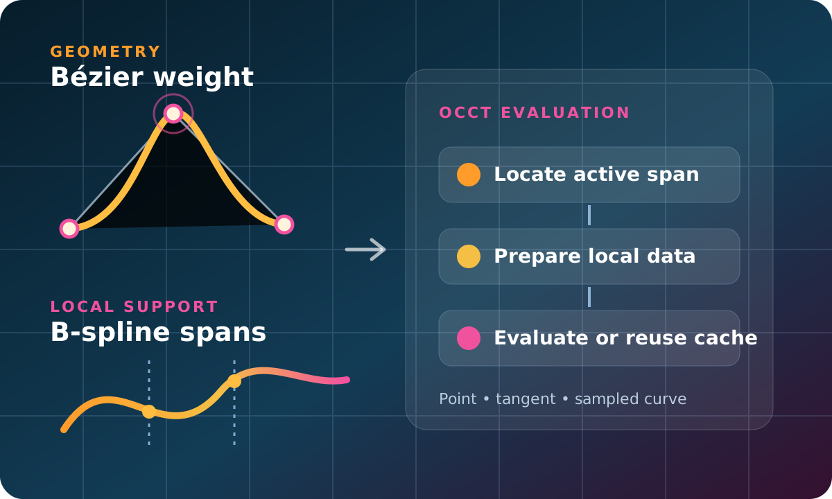
B-splines and Bézier geometry are used throughout Open CASCADE Technology. They appear in imported CAD data, approximation, interpolation, surface construction, offsets, intersections, fillets, meshing, visualization, and many other modeling operations.

Public geometry classes are easy to recognize:

• Geom_BezierCurve
• Geom_BSplineCurve
• Geom_BezierSurface
• Geom_BSplineSurface

NURBS means non-uniform rational B-spline. OCCT does not need a separate NURBS geometry class: a Geom_BSplineCurve or Geom_BSplineSurface with varying weights represents rational B-spline geometry. “Non-uniform” describes knot structure, while “rational” identifies a weighted numerator and denominator. Polynomial B-splines use these classes without varying weights.

Evaluation below these classes is less obvious. A call such as curve->EvalD0(u) can involve knot location, selection of local poles, homogeneous coordinates, polynomial evaluation, rational derivative conversion, or reuse of a current-span cache. Adaptor evaluation has a different cost profile from direct evaluation. A batch evaluator may choose between direct and cached calculation according to sample count and order.

This guide starts with geometry and follows those paths through OCCT’s current implementation. Similar principles apply to their 2D curve counterparts. Interactive examples sit beside their topics and use OCCT for all calculations.

This article begins Deep into Kernel, a series that follows OCCT subjects from mathematical foundations through implementation choices and practical use. Each guide combines source-level explanations, direct links to OCCT reference documentation, and focused interactive examples.

Foundations and terminology

The properties that must stay separate

A key distinction is rational versus non-rational geometry. A rational curve or surface stores a scalar weight with each pole. A non-rational one does not need varying pole weights.

A separate comparison is periodic versus non-periodic geometry. These properties are independent:

• A B-spline can be rational and periodic.
• It can be rational and non-periodic.
• It can be non-rational and periodic.
• It can be non-rational and non-periodic.

An OCCT Bézier curve is non-periodic, but it can still be rational.

OCCT APIs normally call a control point a pole. Both terms are equivalent in this guide. A span is a non-zero interval between consecutive values in an expanded, or flat, knot sequence. Within one span, a non-rational B-spline is one polynomial piece. A rational B-spline is a quotient of polynomial pieces.

The short mental model

A degree p Bézier curve has p + 1 poles and one parameter interval, normally [0, 1]. Every pole contributes across that interval.

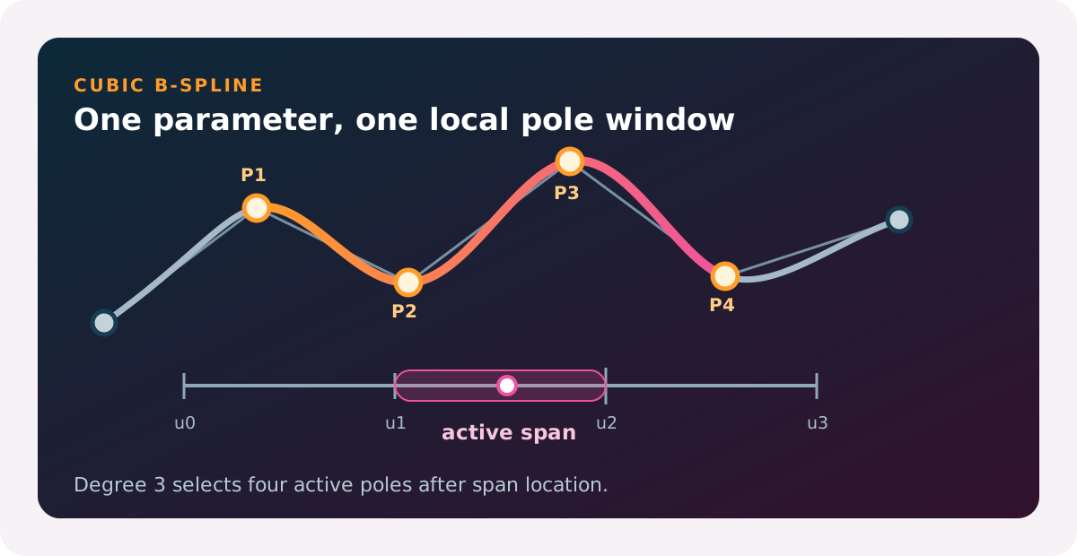
A B-spline adds a knot sequence. Its knots divide the parameter domain into spans. For degree p, only p + 1 nearby poles normally contribute inside a regular span. This local support is the main geometric difference a developer sees when editing a pole.

A Bézier or B-spline surface extends this idea in two directions, u and v. Its poles form a rectangular control net.

An OCCT spline cache stores a polynomial representation of its current span. GeomAdaptor_Curve and GeomAdaptor_Surface use rolling one-entry caches. A curve adaptor remembers one active span. A surface adaptor remembers one active (U span, V span) cell. Crossing a boundary replaces cached coefficients; an adaptor does not retain a table of every span previously visited.

Where the implementation lives

It helps to separate geometry storage from numerical evaluation:

Layer	Main classes or packages	Responsibility
Geometry objects	Geom_BezierCurve, Geom_BSplineCurve, Geom_BezierSurface, Geom_BSplineSurface	Own poles, weights, knots, multiplicities, degree, and periodic flags
Curve mathematics	BSplCLib	Knot handling, B-spline algorithms, Bézier wrappers, and direct curve evaluation
Surface mathematics	BSplSLib	Tensor-product surface evaluation built on spline mathematics
Polynomial helpers	PLib	Polynomial evaluation and rational derivative conversion
Curve cache	BSplCLib_Cache	Prepared polynomial coefficients for one curve span
Surface cache	BSplSLib_Cache	Prepared polynomial coefficients for one surface span cell
Adaptors	GeomAdaptor_Curve, GeomAdaptor_Surface	Type dispatch, local bounds, and lazy cached evaluation
Batch evaluation	GeomGridEval_*	Efficient evaluation of ordered point or derivative grids
Evaluation representations	GeomEval_Rep*	Optional alternative evaluation attached to a geometry object

One geometric curve can therefore be evaluated through several paths:

Geom_BSplineCurve::EvalD0()
  -> BSplCLib::LocateParameter()
  -> BSplCLib::D0()
  -> local B-spline evaluation

GeomAdaptor_Curve::EvalD0()
  -> BSplCLib_Cache
  -> cached polynomial evaluation

GeomGridEval_BSplineCurve::EvaluateGrid()
  -> group ordered parameters by span
  -> direct or cached evaluation for each group

All three paths should agree on their mathematical point. Their setup cost, state ownership, and reuse strategy differ.

Evaluation representations in OCCT 8.x

Current OCCT geometry can carry an optional evaluation representation. Before classic spline evaluation begins, methods such as Geom_BSplineCurve::EvalD0() ask GeomEval_RepUtils whether an attached representation can provide a requested result.

This adds one more branch to our mental model:

Geom_BSplineCurve::EvalD0(u)
  -> attached evaluation representation available?
       yes: evaluate through that representation
       no: continue through BSplCLib

Such a representation is useful when a geometry object has an associated alternative or optimized evaluator. A dynamic type alone therefore does not prove which numerical path was used. When profiling, debugging, or comparing two evaluators, check for an evaluation representation before attributing every call to BSplCLib or a span cache.

Most of this guide focuses on classic evaluation because it directly exposes spline mathematics and cache behavior. Cross-path tests should nevertheless include geometry with and without an attached representation when that feature is relevant to an application.

Bézier curve geometry

Non-rational Bézier curves

A non-rational Bézier curve of degree p is a sum of its poles multiplied by Bernstein basis functions:

C(u) = sum from i=0 to p of B(i,p,u) * P(i),  0 <= u <= 1

B(i,p,u) = binomial(p,i) * u^i * (1-u)^(p-i)

The Bernstein basis has several useful properties on [0, 1]:

• Every basis value is non-negative.
• The basis values sum to one.
• First and last basis functions become one at their corresponding ends.
• The curve stays inside the convex hull of its poles.
• Endpoint tangent directions follow first and last control-polygon edges.

A cubic curve has four poles and normally passes through its first and last poles. Its two middle poles control shape and endpoint tangent directions.

Geom_BezierCurve stores an array of poles, a weight array, a rationality flag, and an optional evaluation representation. Weight storage may exist even when the curve is non-rational. The low-level Weights() helper returns a null pointer for the non-rational case so BSplCLib can select its polynomial path.

The normal invariants are:

Degree() == NbPoles() - 1
FirstParameter() == 0
LastParameter() == 1

A Bézier follows the B-spline evaluator

The regular Geom_BezierCurve::EvalD0(), EvalD1(), EvalD2(), and EvalD3() methods call BSplCLib. The Bézier overloads build the equivalent clamped knot data:

distinct knots   = { 0, 1 }
multiplicities   = { p+1, p+1 }

They then call the shared B-spline evaluation functions. A Bézier is mathematically a B-spline with one span, so this implementation unifies the numerical path. Changes in shared BSplCLib code can consequently affect both geometry classes.

De Casteljau’s construction is still useful for teaching and for understanding the convex combinations. For a cubic curve, one interpolation level is:

Q0 = (1-u) P0 + u P1
Q1 = (1-u) P1 + u P2
Q2 = (1-u) P2 + u P3

The process repeats with Q0, Q1, and Q2 until one point remains. The standard high-level OCCT evaluation path does not need to expose those intermediate levels.

Rational Bézier curves

A rational Bézier adds one weight w(i) per pole:

             sum B(i,p,u) * w(i) * P(i)
C(u) = ------------------------------------------------
                    sum B(i,p,u) * w(i)

OCCT evaluates the numerator and denominator in homogeneous form and converts the result to Cartesian coordinates. A pole can be viewed as the homogeneous value:

H(i) = (w(i) * x(i), w(i) * y(i), w(i) * z(i), w(i))

Evaluation first uses these four-component values, then divides their first three components by the fourth.

Weights control attraction to poles. Increasing one positive weight pulls a curve towards that pole. Decreasing it reduces that pole’s influence. Multiplying every weight by a common non-zero factor leaves geometry unchanged because this factor cancels between numerator and denominator.

Rational Bézier curves can represent conics exactly. This example begins with a quadratic quarter circle:

#include <cmath>

#include <Geom_BezierCurve.hxx>
#include <NCollection_Array1.hxx>
#include <gp_Pnt.hxx>

NCollection_Array1<gp_Pnt> aPoles(size_t{3});
aPoles.ChangeAt(0) = gp_Pnt(1.0, 0.0, 0.0);
aPoles.ChangeAt(1) = gp_Pnt(1.0, 1.0, 0.0);
aPoles.ChangeAt(2) = gp_Pnt(0.0, 1.0, 0.0);

NCollection_Array1<double> aWeights(size_t{3});
aWeights.ChangeAt(0) = 1.0;
aWeights.ChangeAt(1) = 1.0 / std::sqrt(2.0);
aWeights.ChangeAt(2) = 1.0;

occ::handle<Geom_BezierCurve> aCurve =
  new Geom_BezierCurve(aPoles, aWeights);

const gp_Pnt aMidPoint = aCurve->EvalD0(0.5);

With the middle weight equal to 1 / sqrt(2), the curve is an exact unit quarter circle. The point at u = 0.5 is approximately (0.7071, 0.7071, 0). Changing only that middle weight demonstrates the rational part clearly because the poles stay fixed.

High-level Geom constructors require positive weights. Positive weights preserve the conventional convex-hull interpretation in homogeneous form and avoid denominator sign changes inside the normal parameter range.

B-spline curve geometry

Knots create local polynomial pieces

A B-spline curve combines poles using B-spline basis functions:

C(u) = sum N(i,p,u) * P(i)
sum N(i,p,u) = 1

The support of N(i,p,u) is limited to the knot interval from U(i) to U(i+p+1).

For rational geometry, each term also contains a pole weight and the sum is divided by the weighted basis sum, just as for a rational Bézier.

The knot sequence divides the domain into spans. In a regular span, only a local set of p + 1 poles contributes to a degree p curve. This is local support: editing one pole affects only the spans covered by its basis function.

The basis is defined recursively. For degree zero, a basis function is active on one knot interval. Higher degree basis functions blend two lower-degree functions:

N(i,0,u) = 1 when U(i) <= u < U(i+1), otherwise 0

N(i,p,u) = ((u-U(i)) / (U(i+p)-U(i))) * N(i,p-1,u)
         + ((U(i+p+1)-u) / (U(i+p+1)-U(i+1))) * N(i+1,p-1,u)

Terms with a zero denominator are treated as zero. Local evaluation can also be understood through de Boor construction, which repeatedly blends active poles using knot-dependent coefficients. OCCT uses optimized algorithms and data preparation while preserving this locality.

Within its active domain, B-spline basis functions are non-negative and form a partition of unity:

sum N(i,p,u) = 1

Each basis function N(i,p,u) has support only over its knot interval from U(i) to U(i+p+1). These properties explain several familiar geometric results: translating or rotating every pole transforms a curve consistently, a non-rational curve remains inside its active-pole convex hull, and changing one pole has only local influence. With positive rational weights, normalized rational basis functions still form a non-negative weighted average.

This recurrence also explains why a complete pole set is not processed for every value. Once its active span is known, non-zero basis functions form a compact triangular calculation around that span. A degree-three curve needs four active poles for a regular point, whether its complete representation owns eight poles or eight hundred thousand.

De Boor’s algorithm is a B-spline counterpart to de Casteljau’s algorithm. It begins with active p + 1 poles and performs repeated affine combinations. Interpolation factors depend on a parameter and local knots rather than only on a normalized Bézier parameter. Rational geometry permits this construction in homogeneous coordinates.

complete curve data
       |
       v
locate active span
       |
       v
select p + 1 local poles
       |
       v
repeat knot-dependent blends
       |
       v
curve value at u

This is the important performance distinction. Total pole count influences storage and span location, but the arithmetic after location is controlled mainly by the degree and derivative order.

Distinct knots, multiplicities, and flat knots

Geom_BSplineCurve stores distinct knot values and a multiplicity for each value. It also stores a corresponding flat knot sequence used by many low-level operations. Its constructor copies distinct knots and multiplicities, then immediately generates this sequence by repeating each knot according to its multiplicity. Geom_BSplineSurface performs this work independently for U and V directions.

For a cubic curve:

distinct knots = 0 1 2 3
multiplicities = 4 1 1 4
flat sequence  = 0 0 0 0 1 2 3 3 3 3

This preparation is part of a high-level Geom object and is not optional. KnotSequence() returns a sequence already maintained by its curve; UKnotSequence() and VKnotSequence() provide surface equivalents. Operations that change knot representation, including knot insertion, multiplicity changes, and degree changes, rebuild stored sequences. Application code should therefore not build or cache another copy unless a separate representation is genuinely required. For a uniform non-periodic B-spline with multiplicity one at every knot, flat and distinct sequences match.

A Bézier curve has no user-supplied knot array. OCCT represents it with canonical distinct knots {0, 1}, endpoint multiplicities equal to degree + 1, and a flat sequence in which both endpoints occur degree + 1 times. Bézier surfaces use this canonical representation independently in U and V. Common evaluators can therefore consume Bézier and B-spline geometry through one knot-sequence interface.

The non-zero intervals [0, 1], [1, 2], and [2, 3] are the three spans. Repeated values in the flat sequence do not form spans because their interval length is zero.

The parameter domain of a non-periodic clamped B-spline is obtained from the flat sequence after accounting for the degree. It should be read from FirstParameter() and LastParameter() rather than reconstructed in application code.

In current Geom_BSplineCurve implementation, bounds correspond to degree-adjusted entries of a flat sequence. With OCCT’s one-based arrays, use this conceptual rule:

first parameter = flat knot at degree + 1
last parameter  = flat knot at upper index - degree

For this cubic flat sequence, evaluation produces domain [0, 3]. Exposing a flat sequence beside distinct knots helps diagnostic tools show span indices, multiplicities, and boundary conventions simultaneously.

OCCT’s geometry API limits B-spline degree. High degree increases active pole window, temporary storage, evaluation cost, and sensitivity to poor parameter scaling. CAD models commonly use degree two or three, with higher degrees when approximation or construction requires them. More spans are often easier to control than one unnecessarily high-degree piece.

Multiplicity controls continuity

For an interior knot of multiplicity m and a curve of degree p, the common continuity is:

C continuity order = p - m

A simple interior knot on a cubic curve normally gives C2 continuity. Multiplicity two gives C1; multiplicity three gives C0. A multiplicity equal to the degree can create a visible change in tangent direction while the curve remains connected.

This formula describes parametric continuity. C1 means that first derivative vectors agree, including their magnitude. Geometric continuity asks a different question: G1 requires matching tangent directions but permits different parameter speeds. Two pieces can therefore meet with G1 continuity without being C1. Knot multiplicity gives continuity guaranteed by a spline representation; special pole configurations can still produce higher geometric agreement at a particular join.

A B-spline whose interior knots all have degree multiplicity is often described as piecewise Bézier. Each span behaves like a Bézier segment, while the complete object remains one B-spline with shared structure.

Knot insertion differs from moving a pole. Exact knot insertion changes representation without changing geometry. It adds knots and poles to preserve shape with finer local structure. Moving a pole changes shape.

Closed and periodic curves

A curve is closed when its start and end points coincide within tolerance. Periodicity is stronger: the parameterization, pole structure, and knot structure repeat across a period.

A closed non-periodic B-spline may have coincident endpoints but different derivative behavior at those endpoints. A periodic B-spline can be evaluated at parameters outside its principal range after normalization by the period.

The seam is a valuable test location. Compare values and derivatives:

• At the first parameter.
• At the last parameter.
• Just below and above both boundaries.
• At values shifted by one positive or negative period.

This catches errors in normalization, span location, and derivative-side selection that ordinary interior tests do not expose.

Bézier and B-spline surfaces

Tensor-product geometry

A surface applies the curve basis in two parameter directions. For a non-rational B-spline surface:

S(u,v) = sum over i and j of N(i,p,u) * M(j,q,v) * P(i,j)

The poles form a rectangular control net. The u direction has its own degree, knots, multiplicities, and periodic flag. The v direction has another independent set.

A rational surface includes weights in the numerator and denominator:

                  sum N(i,p,u) * M(j,q,v) * w(i,j) * P(i,j)
S(u,v) = ----------------------------------------------------------------
                        sum N(i,p,u) * M(j,q,v) * w(i,j)

The active region is a span cell: one non-zero u interval combined with one non-zero v interval. A degree (p, q) regular cell normally depends on (p + 1) * (q + 1) local poles.

Directional rationality

OCCT surface implementations can identify whether weights vary in the u direction, the v direction, or both. This matters because a surface may have equal weights along one direction while varying along the other. The evaluator can avoid unnecessary rational work where the representation allows it.

Equal weights everywhere describe geometry equivalent to a non-rational surface. They do not always imply that every stored or imported representation has already been simplified to a non-rational form.

Surface derivatives

Surface evaluation can return:

• EvalD0: a point.
• EvalD1: a Geom_Surface::ResD1 containing the point and first derivatives D1U and D1V.
• EvalD2: a Geom_Surface::ResD2 that also contains D2U, D2V, and the mixed derivative D2UV.
• EvalD3: a Geom_Surface::ResD3 that also contains the third-order directional and mixed derivatives.
• EvalDN: one requested derivative order in u and v.

Rational surface derivatives require quotient-rule conversion of a two-dimensional table of homogeneous derivatives. The amount of work grows quickly with derivative order and with the two degrees. A surface performance test should therefore state both degrees and requested derivative matrix.

At a regular surface point, the two first derivatives define the tangent plane. Their cross product gives an oriented normal direction:

normal direction = Su x Sv
unit normal       = (Su x Sv) / |Su x Sv|

The orientation follows the order of the u and v parameters. If Su x Sv is zero or very small, the parameterization is singular or nearly singular at that point and a stable unit normal cannot be obtained by direct normalization. This distinction matters in shading, meshing, offset construction, curvature analysis, and intersection marching.

Direct evaluation in OCCT

Geom_BSplineCurve::EvalD0() step by step

For classic spline path without an overriding evaluation representation, direct point evaluation broadly follows these steps:

1. Normalize the parameter if the curve is periodic.
2. Locate active knot span.
3. Select local portion of the flat knot sequence.
4. Select active poles and optional weights.
5. Call the appropriate BSplCLib evaluator.
6. Convert homogeneous output when the curve is rational.

Conceptually:

Geom_BSplineCurve::EvalD0(u)
  -> BSplCLib::LocateParameter(...)
  -> prepare local knots, poles, and weights
  -> BSplCLib::D0(...)
  -> gp_Pnt

Evaluation-representation checks occur before classic evaluation. A Geom_BSplineCurve object can carry an alternative EvalRepresentation, so its dynamic geometry type alone is not enough to identify numerical code being executed.

EvalD0 needs only a point. EvalD1, EvalD2, and EvalD3 prepare and return a point together with requested derivatives. EvalDN handles an arbitrary requested derivative order. Do not request a higher derivative order when a calling algorithm only needs a point or tangent.

Prefer the result-returning evaluation API

For new application code, prefer EvalD0, EvalD1, EvalD2, EvalD3, and EvalDN when available on a geometry or adaptor. Value(u) and EvalD0(u).Point produce equal points, but EvalD0 states requested derivative order explicitly and follows a naming pattern shared with derivative methods.

The older D0, D1, D2, and D3 methods write into output parameters. Their EvalD* counterparts return the result directly. For example, Geom_Curve::EvalD1() returns Geom_Curve::ResD1, which contains the point and first derivative:

const Geom_Curve::ResD1 aResult = aCurve->EvalD1(aParameter);
const gp_Pnt& aPoint   = aResult.Point;
const gp_Vec& aTangent = aResult.D1;

The result structures are aggregates, so C++17 structured bindings provide a compact alternative when the order is clear:

const auto [aPoint, aTangent] = aCurve->EvalD1(aParameter);

const auto [aSurfacePoint, aDerivativeU, aDerivativeV] =
  aSurface->EvalD1(aU, aV);

Named fields remain useful in longer code where Point, D1, D1U, or D1V communicate the meaning more clearly. Both forms avoid declaring mutable output objects before the evaluation call.

Rational derivative conversion in PLib

For rational curves, OCCT first evaluates derivatives of the weighted coordinates and of the denominator. If A(u) is the weighted coordinate numerator and w(u) is the denominator, then:

C(u) = A(u) / w(u)

First derivative is:

C'(u) = (A'(u) - w'(u) * C(u)) / w(u)

Higher derivatives recursively subtract combinations of lower Cartesian derivatives and denominator derivatives. PLib contains the helpers that perform this conversion for curves and surfaces.

One consequence is that a rational curve can have non-zero Cartesian derivatives above the polynomial degree of its homogeneous numerator and denominator. The quotient itself is not a polynomial. Code should not assume that every derivative above the degree is zero merely because this is true for a polynomial Bézier curve.

Direct Bézier evaluation

The ordinary Bézier path uses the equivalent one-span B-spline structure. This gives a common implementation for knot handling, rational values, and derivatives. It also makes a Bézier a particularly simple cache case: its normal domain never crosses an interior span boundary.

This benchmark uses a degree-nine Geom_BezierCurve. It compares direct EvalD0() calls, repeated GeomAdaptor_Curve::EvalD0() calls, and one GeomGridEval_BezierCurve::EvaluateGrid() call for one ordered parameter set.

Direct surface evaluation

Geom_BSplineSurface prepares local data in both directions and delegates tensor-product work to BSplSLib. For a rational surface it evaluates homogeneous derivative tables and converts them using PLib.

Request the point and both first partial derivatives in one returned result when a tangent plane or normal is needed:

const auto [aPoint, aDerivativeU, aDerivativeV] =
  aSurface->EvalD1(aU, aV);

const gp_Vec aNormalDirection = aDerivativeU.Crossed(aDerivativeV);

The surface path has two span searches and a larger local control net. Access order therefore matters even more than it does for curves. A regular grid that advances monotonically in u and v can reuse local information; random cells can repeatedly replace it.

Local evaluation and derivative sides

At an interior knot, a curve has a polynomial piece on each side. If continuity is lower than requested derivative order, left and right derivatives differ. Local evaluation APIs allow callers to specify an intended knot interval.

This matters at:

• High-multiplicity interior knots.
• Trimmed adaptor boundaries that coincide with a knot.
• The seam of periodic geometry.
• Numerical tests that compare cached and direct evaluation.

A cache represents one polynomial piece. It cannot choose a mathematically ambiguous side on behalf of a calling algorithm. That algorithm must define required boundary behavior.

At a regular curve point, first and second derivatives also provide familiar geometric quantities:

speed     = |C'(u)|
curvature = |C'(u) x C''(u)| / |C'(u)|^3

Speed depends on the chosen parameterization. Curvature is geometric, but the formula becomes numerically unreliable when |C'(u)| is close to zero. Algorithms should detect that degeneracy instead of dividing by a very small cubic denominator.

Curve and surface span caches

What BSplCLib_Cache stores

BSplCLib_Cache prepares one curve span as polynomial coefficients. Its state includes the degree, periodicity information, the parameter interval represented by the cache, rational or non-rational coefficients, and scaling needed to convert local derivatives back to the curve parameter.

Building the cache requires the degree, flat knots, poles, and optional weights. The cache locates the span containing the build parameter and converts that local B-spline piece into a form that can be evaluated repeatedly.

For a non-rational 3D curve, each polynomial coefficient contains three scalar components. A rational curve needs four homogeneous components:

X * weight, Y * weight, Z * weight, weight

Associated cache parameters record degree, periodic flag, valid parameter interval, current span index, span start, and span length. Broad build and evaluation flow is:

BuildCache(u)
  -> normalize a periodic parameter when necessary
  -> locate active span
  -> select its knots, poles, and optional weights
  -> prepare polynomial coefficient rows

Repeated D0/D1/D2/D3 calls
  -> map global u to local parameter
  -> evaluate the prepared polynomial with PLib
  -> rescale derivatives to the global parameter
  -> convert homogeneous derivatives when rational

Repeated calls therefore avoid span search, local pole extraction, local knot preparation, and spline-to-polynomial conversion. They do not avoid polynomial evaluation itself.

This cache does not observe its source geometry object. If poles, weights, knots, degree, or periodic structure change, its owner must rebuild it. A valid parameter interval only says that a parameter belongs to a cached span; it does not prove that coefficients still describe current geometry revision.

Curve cache parameterization

A cached curve span uses a local parameter in [0, 1]:

t = (u - u0) / (u1 - u0)

where [u0, u1] denotes a source span. A derivative with respect to t does not equal a derivative with respect to u. Conversion includes powers of inverse span length:

d/d u       = (1 / spanLength)   * d/d t
d2/d u2     = (1 / spanLength^2) * d2/d t2
d3/d u3     = (1 / spanLength^3) * d3/d t3

This scaling is especially important for small spans. A tiny span can produce large parameter derivatives even when the 3D curve looks visually smooth.

A rational cache stores numerator and denominator polynomial information. It evaluates them at a local parameter and applies rational conversion before returning Cartesian results.

Cache validity

IsCacheValid(u) answers whether u belongs to the prepared parameter interval under the cache’s boundary rules. A robust owner must also track geometry changes.

A useful ownership model is:

cache key = geometry revision + span identity + evaluation settings

Geometry revision changes after an edit. Span identity changes when a parameter crosses a boundary. Evaluation settings must record intended derivative side where that distinction matters.

Near a knot, floating-point comparisons can otherwise cause an unstable choice between neighboring pieces. Cache parameters account for periodic normalization and first and last spans, then apply boundary rules when checking whether a requested parameter still belongs to its current entry. Application code should use cache validity operations rather than recreate these comparisons with an arbitrary epsilon.

A diagnostic display can make cache behavior explicit:

parameter       1.723
normalized      1.723
span            [1.50, 2.00]
local parameter 0.446
action          reuse

After crossing the knot it may become:

parameter       2.004
normalized      2.004
span            [2.00, 2.35]
local parameter 0.0114
action          rebuild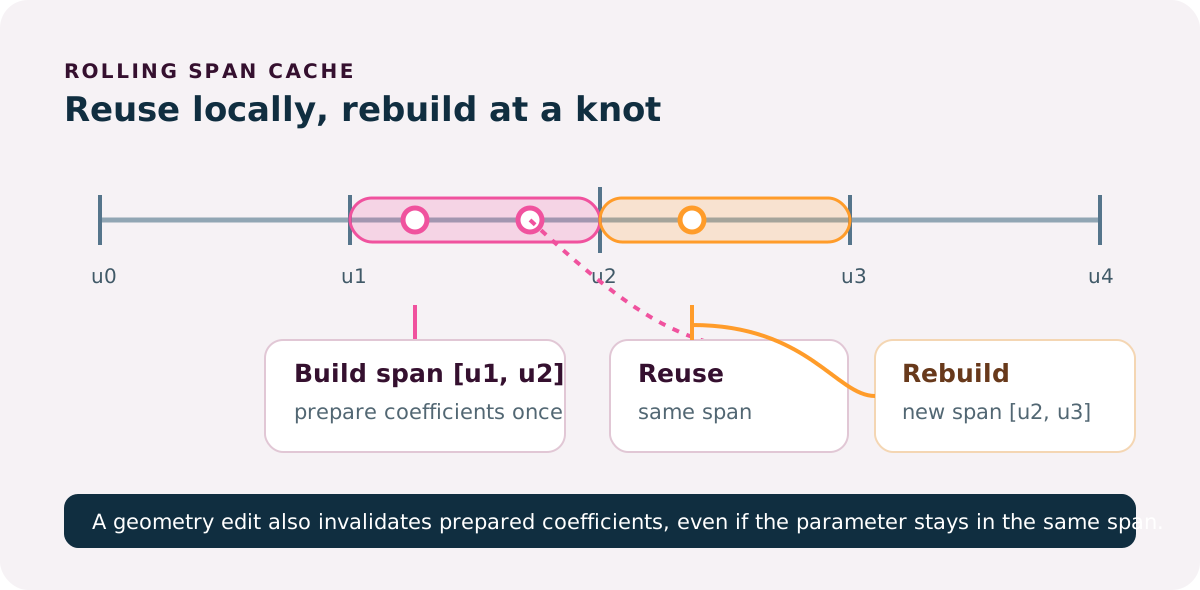

BSplSLib_Cache and a surface cell

The surface cache represents one (u, v) span cell. It stores a tensor-product polynomial patch and optional rational information. Its local coordinates are centered:

uLocal = (u - uMid) / ((u1 - u0) / 2)
vLocal = (v - vMid) / ((v1 - v0) / 2)

The cell therefore uses [-1, 1] x [-1, 1], unlike the curve cache’s [0, 1] interval. This difference is an OCCT implementation detail worth remembering when reading the two cache classes.

Surface evaluation proceeds through one direction and then the other, using the prepared coefficient grid. Rational surface evaluation additionally computes and converts the denominator derivative table. Because a cell can contain many coefficients, rebuilding a rational surface cache can be significantly more expensive than evaluating one isolated point directly.

The cached coefficients form a bivariate polynomial. OCCT evaluates one direction into intermediate data and then evaluates the other direction. The implementation can choose the higher-degree direction first to reduce intermediate work for asymmetric degrees. For a bicubic surface the difference is small; for degrees such as three by ten, evaluation order can be more significant.

A non-rational first-derivative request needs the value and the two directional derivatives. Rational evaluation also needs compatible numerator and denominator derivative data for the quotient recurrence. Second derivatives add pure and mixed terms. Preserving the correct rationality classification avoids carrying that extra work into surfaces that do not need it.

When caching helps

Caching is an investment. It helps when the build cost is recovered through reuse.

Access pattern	Likely choice
One isolated point	Direct geometry evaluation
Many nearby points in one span	Adaptor or explicit span cache
Ordered plotting across the curve	Grid evaluator
Parameters alternating between distant spans	Direct evaluation or grouping before caching
Regular surface grid	Surface grid evaluator
Random surface cells	Measure direct evaluation against any cache policy

The correct choice depends on degree, rationality, derivative order, span count, and sample distribution. There is no universal rule that a cache is always faster.

Adaptors, cache ownership, and threads

GeomAdaptor_Curve as a rolling one-span cache

GeomAdaptor_Curve provides one interface for lines, circles, ellipses, Bézier curves, B-splines, offsets, and other curve types. Elementary geometry can dispatch to analytic evaluators. Bézier and B-spline evaluation can use a mutable BSplCLib_Cache.

For a B-spline, its adaptor keeps one currently active span:

call in S2   build S2
call in S2   reuse S2
call in S3   replace cache with S3
call in S3   reuse S3
call in S2   replace cache with S2 again

There is no least-recently-used table and no array of prepared spans. The policy favors parametric locality. Algorithms that advance gradually through the parameter usually reuse the entry. Algorithms that alternate between spans can rebuild it on most calls.

Curve adaptor evaluation state

For ordinary B-spline evaluation, the broad EvalD0() state machine is:

GeomAdaptor_Curve::EvalD0(u)
  -> is u an exact adaptor boundary?
       yes: choose local interval and use LocalD0
  -> is the cache missing or invalid for u?
       yes: rebuild it for u
  -> BSplCLib_Cache::D0(u)

EvalD1, EvalD2, and EvalD3 reuse a rolling-cache approach for ordinary interior evaluation. General EvalDN evaluation uses a direct path because a curve cache exposes standard derivatives rather than every arbitrary order.

A Bézier has only one normal span. After its first cache build, movement from u = 0 to u = 1 stays inside one interval. This makes Bézier evaluation a clean case for understanding reuse before studying B-spline transitions.

Bounds, copies, and geometry mutation

An adaptor owns first and last parameters. At an exact bound that coincides with a knot, it uses local evaluation to select an intended interval. Correct derivative-side selection is more important than forcing every call through its cache.

Load() establishes the geometry and bounds and clears spline cache state when necessary. ShallowCopy() shares underlying immutable geometry but gives the copy its own cache state. This is useful for worker-local evaluation.

If application code mutates geometry behind an adaptor, it must reload or reconstruct that adaptor before relying on cached results. Another handle to this curve object does not provide automatic cache invalidation.

GeomAdaptor_Surface

The surface adaptor holds one active (U span, V span) cell for B-spline surfaces. Movement within that cell can reuse BSplSLib_Cache. Crossing a knot in either direction replaces it.

The common EvalD0, EvalD1, and EvalD2 paths can use the surface cache. Higher-order paths such as EvalD3 and general EvalDN use different direct evaluation routes. A Bézier surface has one cell over its normal domain, so it provides the simplest surface-cache workload.

Access order matters strongly for surfaces. Row-major or column-major movement across a grid changes one span direction predictably. A random (u, v) sequence can replace the one-cell cache frequently.

Const evaluation is not immutable

Adaptor evaluation methods are const in their public interface, but cache handles and cached state are mutable. Two threads calling EvalD0() on a shared B-spline adaptor can race while rebuilding or replacing its cache.

The preferred parallel pattern is one adaptor per worker:

GeomAdaptor_Curve aBaseAdaptor(aCurve);

// Create or shallow-copy one adaptor for each worker.
auto aWorkerAdaptor =
  occ::down_cast<GeomAdaptor_Curve>(aBaseAdaptor.ShallowCopy());

The geometry may be shared while it remains immutable. Each worker owns its adaptor and cache. Other safe patterns include direct evaluation on immutable geometry, explicit worker-local caches, or external synchronization when sharing cannot be avoided.

A const reference exposes only the adaptor’s const API; it does not make the internal cache immutable.

Consider a shared adaptor whose cache currently describes span S1:

thread A calls EvalD0() in S2
thread B calls EvalD0() in S3

Both threads can observe an invalid cache and begin rebuilding it. One can replace span parameters while another prepares or evaluates coefficients. This race also affects a surface adaptor, whose mutable state contains both u and v spans plus a coefficient grid for that cell.

The common safe patterns are:

• Construct a task-local adaptor from shared immutable geometry.
• Use ShallowCopy() and keep the resulting adaptor private to one worker.
• Construct a task-local GeomGridEval_* object for a known sample batch.
• Use direct geometry evaluation when cache reuse is too low to justify stateful adaptors.
• Serialize a shared adaptor only when worker-local ownership is impractical and the cost is acceptable.

A mutex can make shared calls safe, but it serializes the evaluation hot path. Separate adaptors normally express the ownership more clearly and preserve useful parallelism.

Batch and grid evaluation

GeomGridEval_BSplineCurve

GeomGridEval_BSplineCurve is designed for many parameter values. It determines active spans, groups ordered samples by span, and decides whether a local cache is worthwhile for each group.

Current source uses a small cache threshold. A group containing one sample can use direct BSplCLib evaluation. A group with enough samples builds BSplCLib_Cache and reuses it. The exact threshold is an implementation choice and may evolve after benchmarking; the stable principle is that cache construction should be paid for by reuse.

Once span start and length are known, a grid evaluator can calculate a local parameter and call local cache entry points. It does not need to ask its cache to rediscover information already known by a batch loop.

This class fits:

• Curve plotting and tessellation.
• Sampling for extrema bracketing.
• Numerical integration grids.
• Visualization.
• Export of sampled geometry.
• A curve visualizer that requests hundreds of points at once.

B-spline benchmark uses one cubic curve with four polynomial spans. Changing sample count changes density within those spans without changing curve geometry.

GeomGridEval_BSplineSurface

A surface grid evaluator accepts arrays of u and v parameters and evaluates their Cartesian product. It groups work by active span cell. D0, D1, and D2 can use BSplSLib_Cache; higher derivative paths use applicable direct evaluators.

This is a strong fit for surface visualization. A regular parameter grid naturally contains many samples per cell, gives the evaluator enough context to group work by span, and returns the Cartesian product in one operation.

Bézier grid evaluation

GeomGridEval_BezierCurve builds one curve cache for a single Bézier span and reuses it for requested parameters. GeomGridEval_BezierSurface reuses this approach for one polynomial patch. These classes are useful even though they do not have to group several knot spans.

Surface benchmark below uses a degree-six by degree-six Geom_BezierSurface. Unlike a multi-span B-spline surface benchmark later in this guide, this workload stays inside one polynomial patch for an entire grid.

Parameter order is part of the workload

Current B-spline grid implementation assumes that non-periodic parameters progress through spans in ascending order. This ordering is natural for plotting and regular grids.

An arbitrary sequence such as:

0.2, 5.8, 1.4, 9.0, 0.7

does not satisfy ordered-input requirements. A forward-moving fast path cannot assume that a later array element belongs to its current span or a later span.

Use one of these strategies:

• Supply monotonically increasing parameter arrays.
• Sort the parameters and restore requested output order afterward.
• Use independent direct or adaptor evaluation for genuinely random queries.

Implementation contains this precondition, but public evaluator headers do not currently express it clearly. Until API documentation and implementation are aligned, callers should treat ascending order as required. This requirement belongs in tests and API documentation because an array type alone cannot express it.

Performance choices and cost model

Which path should be the default?

Use the highest-level path that matches the workload:

Workload	Good starting point
One point or derivative	Geom_*::EvalD*()
Evaluation through a general algorithm interface	GeomAdaptor_Curve or GeomAdaptor_Surface
Many ordered curve points	GeomGridEval_BSplineCurve or GeomGridEval_BezierCurve
Regular surface grid	GeomGridEval_BSplineSurface or Bézier equivalent
Controlled inner loop with explicit state ownership	BSplCLib_Cache or BSplSLib_Cache
Parallel sampling	One adaptor or cache per worker

Manual caching should rarely be a first optimization. It adds revision tracking, span-boundary behavior, derivative scaling, and thread-ownership responsibilities. Start with direct or adaptor evaluation, measure an actual workload, and move lower only when profiling justifies it.

Sources of curve-evaluation cost

The total cost can include:

1. Parameter normalization for periodic geometry.
2. Span location in the knot sequence.
3. Selection and copying or referencing of local poles and weights.
4. Preparation of local polynomial coefficients.
5. Polynomial or rational evaluation.
6. Derivative conversion and scaling.
7. Repeated calls across an expensive language or process boundary.

For one point, cache construction may cost more than the setup it avoids. For hundreds of ordered points in one span, the build cost can be amortized effectively.

Rational versus non-rational cost

A non-rational evaluator processes three coordinate components. A rational evaluator also processes the denominator and applies quotient-rule conversion. The difference grows with derivative order.

Equal stored weights can describe non-rational geometry, but the actual cost depends on whether the object and evaluator recognize and use the non-rational representation. When performance matters, inspect IsRational() and the low-level weight pointer rather than inferring behavior only from the input file.

If every active weight equals k, that common factor cancels:

       k * sum N(i,p,u) * P(i)
C(u) = ------------------------- = sum N(i,p,u) * P(i)
           k * sum N(i,p,u)

This equality follows from partition of unity. OCCT uses rationality checks to avoid unnecessary homogeneous evaluation when a representation is polynomial. Lower-level preparation can also recognize an active pole window whose weights are equal even if weights vary elsewhere on a complete curve.

Span location and degree

Span location can become visible when many isolated random parameters are evaluated on a curve with many knots. Ordered evaluation reduces that cost because an existing span often remains valid or advances predictably.

Degree changes active problem size. A degree p curve span normally uses p + 1 poles. A degree (p, q) surface cell uses roughly (p + 1) * (q + 1) poles before rational work. High-degree surfaces therefore amplify both preparation and derivative costs.

Benchmark the policy, not only the function

A useful benchmark states:

• Curve or surface type.
• Degree in each direction.
• Number of poles, knots, and spans.
• Rationality and periodicity.
• Derivative order.
• Parameter order.
• Samples per span or cell.
• Cache lifetime and ownership.
• Whether language boundaries are crossed per point or per batch.

Without those details, a result called “cached” or “direct” is difficult to interpret.

Practical OCCT examples

The examples below use the zero-based NCollection_Array1 and NCollection_Array2 interfaces introduced for size_t indexing. Construct an owned zero-based array with its size, iterate from zero to Size(), read with At(), and write with ChangeAt(). These accessors use a zero-based offset even when an array received from another API has different stored lower bounds.

Non-rational Bézier curve

#include <Geom_BezierCurve.hxx>
#include <NCollection_Array1.hxx>
#include <gp_Pnt.hxx>

NCollection_Array1<gp_Pnt> aPoles(size_t{4});
aPoles.ChangeAt(0) = gp_Pnt(0.0, 0.0, 0.0);
aPoles.ChangeAt(1) = gp_Pnt(1.0, 2.0, 0.0);
aPoles.ChangeAt(2) = gp_Pnt(3.0, 2.0, 0.0);
aPoles.ChangeAt(3) = gp_Pnt(4.0, 0.0, 0.0);

occ::handle<Geom_BezierCurve> aCurve =
  new Geom_BezierCurve(aPoles);

const gp_Pnt aPoint = aCurve->EvalD0(0.35);

Useful values for inspection are Degree(), NbPoles(), IsRational(), Poles(), and WeightsArray().

Cubic non-rational B-spline

This curve has six poles, degree three, and three spans:

#include <Geom_BSplineCurve.hxx>
#include <NCollection_Array1.hxx>
#include <gp_Pnt.hxx>

NCollection_Array1<gp_Pnt> aPoles(size_t{6});
aPoles.ChangeAt(0) = gp_Pnt(0.0, 0.0, 0.0);
aPoles.ChangeAt(1) = gp_Pnt(1.0, 2.0, 0.0);
aPoles.ChangeAt(2) = gp_Pnt(2.0, 3.0, 0.0);
aPoles.ChangeAt(3) = gp_Pnt(4.0, 2.0, 0.0);
aPoles.ChangeAt(4) = gp_Pnt(5.0, 0.0, 0.0);
aPoles.ChangeAt(5) = gp_Pnt(6.0, 1.0, 0.0);

NCollection_Array1<double> aKnots(size_t{4});
aKnots.ChangeAt(0) = 0.0;
aKnots.ChangeAt(1) = 1.0;
aKnots.ChangeAt(2) = 2.0;
aKnots.ChangeAt(3) = 3.0;

NCollection_Array1<int> aMultiplicities(size_t{4});
aMultiplicities.ChangeAt(0) = 4;
aMultiplicities.ChangeAt(1) = 1;
aMultiplicities.ChangeAt(2) = 1;
aMultiplicities.ChangeAt(3) = 4;

occ::handle<Geom_BSplineCurve> aCurve =
  new Geom_BSplineCurve(aPoles,
                        aKnots,
                        aMultiplicities,
                        3,
                        false);

const auto [aPoint, aTangent] = aCurve->EvalD1(1.25);

Its flat knot sequence is:

0 0 0 0 1 2 3 3 3 3

Cached evaluation through an adaptor

#include <GeomAdaptor_Curve.hxx>

GeomAdaptor_Curve anAdaptor(aCurve);

for (double aParameter : aParameters)
{
  const gp_Pnt aPoint = anAdaptor.EvalD0(aParameter);
  // Consume aPoint here.
}

For a B-spline, consecutive values in one span reuse prepared coefficients. Crossing a knot rebuilds the one-entry cache. Returning to an older span rebuilds it again.

Curve batch evaluation

#include <GeomGridEval_BSplineCurve.hxx>

NCollection_Array1<double> aParameters(size_t{1000});
const double aFirst = aCurve->FirstParameter();
const double aLast  = aCurve->LastParameter();

for (size_t anIndex = 0; anIndex < aParameters.Size(); ++anIndex)
{
  const double aRatio =
    static_cast<double>(anIndex)
    / static_cast<double>(aParameters.Size() - 1);

  aParameters.ChangeAt(anIndex) = aFirst + aRatio * (aLast - aFirst);
}

GeomGridEval_BSplineCurve anEvaluator(aCurve);
NCollection_Array1<gp_Pnt> aPoints =
  anEvaluator.EvaluateGrid(aParameters);

for (size_t anIndex = 0; anIndex < aPoints.Size(); ++anIndex)
{
  const gp_Pnt& aPoint = aPoints.At(anIndex);
  // Consume aPoint here.
}

If tangents are also needed, request a D1 grid type so point and derivative data are calculated in one batch.

Explicit low-level curve cache

Use an explicit cache only when the surrounding algorithm owns its lifecycle. Unlike the high-level geometry and adaptor APIs, BSplCLib_Cache exposes D0 with an output parameter, so the general EvalD* recommendation does not apply to this low-level interface:

#include <BSplCLib_Cache.hxx>

const auto& aFlatKnots = aCurve->KnotSequence();
const auto& aPoles     = aCurve->Poles();
const auto* aWeights   = aCurve->Weights();

occ::handle<BSplCLib_Cache> aCache =
  new BSplCLib_Cache(aCurve->Degree(),
                     aCurve->IsPeriodic(),
                     aFlatKnots,
                     aPoles,
                     aWeights);

double aParameter = 1.25;
aCache->BuildCache(aParameter, aFlatKnots, aPoles, aWeights);

gp_Pnt aPoint;
aCache->D0(aParameter, aPoint);

aParameter = 1.30;
if (!aCache->IsCacheValid(aParameter))
{
  aCache->BuildCache(aParameter, aFlatKnots, aPoles, aWeights);
}
aCache->D0(aParameter, aPoint);

If a curve changes, rebuild its cache even when a new parameter remains inside an existing interval.

Surface grid evaluation

#include <GeomGridEval_BSplineSurface.hxx>

NCollection_Array1<double> aUParameters(size_t{200});
NCollection_Array1<double> aVParameters(size_t{120});

// Fill both arrays in ascending order inside the surface bounds.

GeomGridEval_BSplineSurface anEvaluator(aSurface);
NCollection_Array2<gp_Pnt> aGrid =
  anEvaluator.EvaluateGrid(aUParameters, aVParameters);

for (size_t aUIndex = 0; aUIndex < aUParameters.Size(); ++aUIndex)
{
  for (size_t aVIndex = 0; aVIndex < aVParameters.Size(); ++aVIndex)
  {
    const gp_Pnt& aPoint = aGrid.At(aUIndex, aVIndex);
    // Consume aPoint here.
  }
}

The returned array is the Cartesian product of the two parameter arrays. At(uIndex, vIndex) addresses it with zero-based row and column offsets, independent of its stored lower bounds. Use ChangeAt(uIndex, vIndex) when mutable access is required. Keep the traversal order consistent with the consumer so memory access remains predictable.

Numerical and API details

Small knot spans

Small spans are not automatically invalid. They may be created by approximation, import, or local refinement. They do make derivative scaling more sensitive because inverse powers of the span length are involved.

Tests should compare direct and cached results on small spans using tolerances appropriate for derivative magnitude. Rejecting a span through an arbitrary absolute length threshold can discard valid geometry. Any protection should follow the algorithm’s tolerance policy rather than a convenient constant.

Parameters exactly on knots

A point value is normally unambiguous where the curve is continuous. Derivatives may not be. At a knot, span location and boundary conventions decide which polynomial piece is used.

Test exact knot values separately from nearby values. A parameter one floating-point step below a knot, exactly equal to it, and one step above it can exercise three different branches.

Poles are not sampled curve points

Except for clamped ends and special configurations, a B-spline does not pass through its poles. A UI should draw its control polygon and sampled curve as different objects. Labeling poles as curve samples gives users an incorrect model of local support and interpolation.

Parameter is not arc length

Equal parameter increments do not normally produce equal distances along a Bézier or B-spline curve. A parameter interval containing strong bending or a high local speed can cover much more geometric distance than another interval of equal length.

Uniform parameter sampling is appropriate for inspecting the evaluator and for workloads whose parameter grid is already prescribed. It is not automatically a uniform geometric tessellation. When approximately equal distances along a curve are required, use an arc-length-aware tool such as GCPnts_UniformAbscissa, or adapt the sampling density using geometric error and derivative information. GCPnts_AbscissaPoint can be used when a point must be found at a requested curvilinear distance from another parameter.

Knot insertion and shape editing

Exact knot insertion preserves the curve while changing the representation. Moving a pole, changing a weight, or changing a knot value normally changes the curve. Code should identify whether an operation is representational or geometric.

This distinction also affects revisions. A shape-preserving representation change can still invalidate a cache because local coefficients and span structure have changed.

Degree elevation

Degree elevation can preserve shape while increasing degree and pole count. It changes local evaluation and cache-construction cost. A performance comparison must not treat an elevated representation as equivalent work merely because it produces matching points.

Reversal

Reversing a spline changes its parameter direction and transforms its knots. Points should match the original curve under the reversed parameter mapping, while odd derivatives change sign according to the chain rule.

Useful tests compare:

original.EvalD0(u)
reversed.EvalD0(reversedParameter(u))

and perform required derivative sign checks.

Isoparametric curves

Fixing one parameter of a B-spline surface produces an isoparametric curve in the other direction. These curves provide a useful cross-check between surface evaluation and curve evaluation. A surface point S(u, vFixed) should agree with the value of the extracted or constructed u isoparametric curve at u.

Source reading map

The implementation spans the Foundation Classes and Modeling Data modules, primarily through the TKMath and TKG3d toolkits.

Reference documentation

The table below collects the package and class reference pages used throughout this guide, including the types that appear only in the C++ examples.

Role	Package reference	Classes used in this guide
Geometry objects	Geom	Geom_BezierCurve, Geom_BSplineCurve, Geom_BezierSurface, Geom_BSplineSurface
Curve evaluation and caching	BSplCLib	BSplCLib_Cache
Surface evaluation and caching	BSplSLib	BSplSLib_Cache
Polynomial evaluation	PLib	Package functions are documented on the package reference page.
Geometry adaptors	GeomAdaptor	GeomAdaptor_Curve, GeomAdaptor_Surface
Evaluation representations	GeomEval	Representation interfaces and utilities are documented through the package reference.
Batch evaluation	GeomGridEval	GeomGridEval_BezierCurve, GeomGridEval_BSplineCurve, GeomGridEval_BezierSurface, GeomGridEval_BSplineSurface
Arrays and control points	NCollection, gp	NCollection_Array1, NCollection_Array2, gp_Pnt
Object handles	Standard	occ::handle

Source directories

Main implementation areas in current source tree are:

Geometry storage

• src/ModelingData/TKG3d/Geom/Geom_BezierCurve.*
• src/ModelingData/TKG3d/Geom/Geom_BSplineCurve.*
• src/ModelingData/TKG3d/Geom/Geom_BezierSurface.*
• src/ModelingData/TKG3d/Geom/Geom_BSplineSurface.*

Curve and surface mathematics

• src/FoundationClasses/TKMath/BSplCLib/
• src/FoundationClasses/TKMath/BSplSLib/
• src/FoundationClasses/TKMath/PLib/

Caches and adaptors

• src/FoundationClasses/TKMath/BSplCLib/BSplCLib_Cache.*
• src/FoundationClasses/TKMath/BSplSLib/BSplSLib_Cache.*
• src/ModelingData/TKG3d/GeomAdaptor/GeomAdaptor_Curve.*
• src/ModelingData/TKG3d/GeomAdaptor/GeomAdaptor_Surface.*

Batch evaluators

• src/ModelingData/TKG3d/GeomGridEval/GeomGridEval_BezierCurve.*
• src/ModelingData/TKG3d/GeomGridEval/GeomGridEval_BSplineCurve.*
• src/ModelingData/TKG3d/GeomGridEval/GeomGridEval_BezierSurface.*
• src/ModelingData/TKG3d/GeomGridEval/GeomGridEval_BSplineSurface.*

Focused tests

These tests are useful starting points when changing evaluation or cache behavior:

• src/FoundationClasses/TKMath/GTests/BSplCLib_Cache_Test.cxx
• src/FoundationClasses/TKMath/GTests/BSplSLib_Cache_Test.cxx
• src/ModelingData/TKG3d/GTests/GeomGridEval_Curve_Test.cxx
• src/ModelingData/TKG3d/GTests/GeomGridEval_BezierCurve_Test.cxx
• src/ModelingData/TKG3d/GTests/GeomGridEval_BezierSurface_Test.cxx
• src/ModelingData/TKG3d/GTests/GeomGridEval_BSplineSurface_Test.cxx

The exact internal path can evolve with OCCT. Read the headers and focused tests from the version used by your application before depending on a threshold or internal representation. The lasting design is the separation of geometry storage, span selection, local evaluation, cache ownership, and batch order.

Compact formula and usage reference

Curve definitions

A non-rational Bézier curve is:

C(u) = sum B(i,p,u) * P(i)

A rational Bézier curve is:

       sum B(i,p,u) * w(i) * P(i)
C(u) = --------------------------------
             sum B(i,p,u) * w(i)

A non-rational B-spline curve replaces the Bernstein basis with the knot-dependent B-spline basis:

C(u) = sum N(i,p,u) * P(i)

Its rational form is:

       sum N(i,p,u) * w(i) * P(i)
C(u) = --------------------------------
             sum N(i,p,u) * w(i)

Surface definitions

A tensor-product B-spline surface is:

S(u,v) = sum N(i,p,u) * M(j,q,v) * P(i,j)

The rational form divides the weighted numerator by its scalar denominator:

           sum N(i,p,u) * M(j,q,v) * w(i,j) * P(i,j)
S(u,v) = ---------------------------------------------------
                 sum N(i,p,u) * M(j,q,v) * w(i,j)

At a regular point, an oriented normal direction is Su x Sv. A unit normal exists only when that cross product has non-zero magnitude.

Continuity and local parameters

For an interior knot of multiplicity m in a degree-p B-spline, the usual parametric continuity is C^(p-m).

The curve cache maps a global span [u0, u1] to [0, 1]:

t = (u - u0) / (u1 - u0)

The surface cache uses a centered coordinate in each direction:

uLocal = (u - (u0 + u1) / 2) / ((u1 - u0) / 2)

which maps a span to [-1, 1]. This rule also applies in v.

For a rational curve written as C = A / w, the first derivative can be written as:

C' = (A' - w' * C) / w

Higher derivatives reuse this quotient relationship recursively. Rational derivatives therefore require denominator derivative data and can remain non-zero at derivative orders above polynomial degrees of A and w.

Evaluation rules

Keep these rules close to spline code:

• Rationality and periodicity are independent properties.
• A curve cache represents one active span; a surface cache represents one active span cell.
• A parameter inside the cached interval does not prove that the cached geometry revision is current.
• At a discontinuous derivative boundary, a calling algorithm must select its intended side.
• A const adaptor evaluation can mutate its internal cache.
• Share immutable geometry across workers, but give each worker its own adaptor or cache.
• Preserve ordered parameter arrays when using a grid evaluator.
• Do not assume that equal parameter steps produce equal distances along a curve.
• Compare direct, cached, adaptor, and batch results before accepting an optimization.

Final perspective

Bézier and B-spline classes expose a compact public API, but efficient and correct evaluation depends on several independent decisions. Rationality determines whether homogeneous conversion is needed. Knots and multiplicities determine local pieces and continuity. Periodicity determines parameter normalization and seam behavior. Adaptors add mutable rolling caches. Grid evaluators exploit ordered batches. Geometry edits determine when every prepared representation becomes stale.

For application code, begin with public geometry or adaptor APIs and measure before adding manual cache ownership. For visualization and dense sampling, evaluate points in batches. For parallel work, share immutable geometry but not mutable adaptor state. For OCCT development, test direct, cached, adaptor, and grid paths against one another at spans, knots, edits, and periodic seams.

Those rules make spline code easier to reason about even when its underlying evaluator changes.

Continue Deep into Kernel

Future articles will examine more of OCCT’s modeling and topology internals. Candidate subjects include offsets, surfaces of revolution, and extrusion. If there is an OCCT area you would like the series to cover, or if you would like to contribute a technical article, use the OCCT3D contact form.