

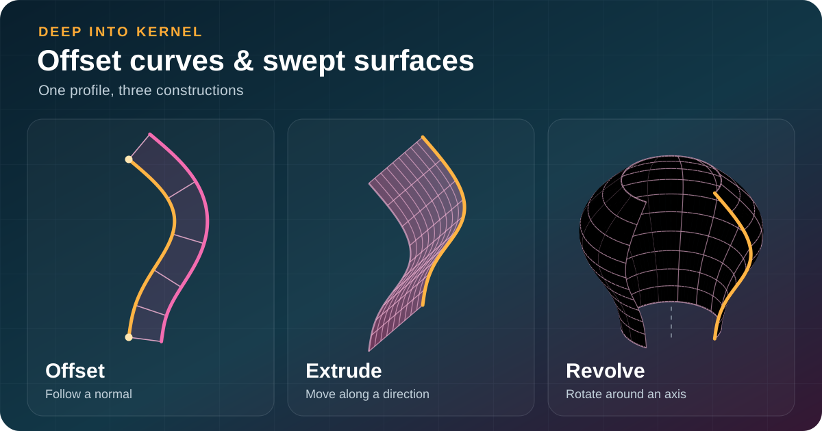
Suppose you already have a curve that describes a part’s profile. You want to turn it into a surface, or create another curve a fixed distance away from it. Fitting another spline would introduce an approximation. OCCT offers a way to keep an exact definition instead.
OCCT can retain an original curve and describe what happens to it. Moving a profile along a straight direction gives an extrusion. Rotating it around an axis gives a surface of revolution. Following a perpendicular direction gives an offset. Each resulting geometry remembers its basis and evaluates points from that definition.
This Deep into Kernel guide follows those operations from a developer’s point of view: what to construct, which parameters to pass, and what to check when a result looks wrong. It continues B-spline and Bezier Geometry in OCCT. A spline can serve as a starting profile, but these ideas also apply to lines, circles, and other supported curves.
Start with four constructions and try their interactive examples. Drag pink handles to edit geometry: numbered poles reshape a profile, patch corners change height, and R changes a cylinder’s radius. Orange d handles change offset distance. Drag empty space to rotate a surface, or use sliders to move its probe.
Each example has Reset example and an expandable How to use note. Reset restores its initial geometry, including singular parameter cases discussed below. You can also select a handle from its menu, focus the view, and use arrow keys to edit it. Open full page gives more room in a separate tab without losing your place here.
Later sections cover choosing an evaluator and reusing work across many points. Derivations and internal recovery paths are optional reading.
One profile, several kinds of geometry
What OCCT means by a basis
A basis curve supplies geometry for another construction. A basis surface serves that role for a surface offset. Both are ordinary OCCT geometry objects; evaluation uses their geometric definitions rather than a sampled mesh.
For example, a swept surface with a B-spline basis still uses that B-spline’s knots, weights, and evaluation methods. It remains a swept-surface object rather than becoming a B-spline surface with its own control net. This distinction matters when editing, choosing an evaluator, or checking what can be represented exactly.
Four classes cover these operations:
| Operation | OCCT class | What you supply |
|---|---|---|
| Move a profile along a straight direction | Geom_SurfaceOfLinearExtrusion | A curve and a direction |
| Rotate a profile about an axis | Geom_SurfaceOfRevolution | A curve and an axis |
| Offset a curve | Geom_OffsetCurve | A curve, a distance, and a reference direction |
| Offset a surface | Geom_OffsetSurface | A surface and a distance |
These classes define geometry. A finite face, a closed shell, or a valid solid involves additional topology. Turning a Geom_SurfaceOfLinearExtrusion into an extruded solid requires faces, end caps, and their connections.
A profile we can reuse
Consider a cubic Bezier curve in the XZ plane. Its four poles give a rounded profile that rises from Z = 0 to Z = 2 while staying away from the Z axis:
#include <Geom_BezierCurve.hxx>
#include <NCollection_Array1.hxx>
#include <gp_Pnt.hxx>

NCollection_Array1<gp_Pnt> aPoles(size_t{4});
aPoles.ChangeAt(0) = gp_Pnt(1.0, 0.0, 0.0);
aPoles.ChangeAt(1) = gp_Pnt(2.0, 0.0, 0.5);
aPoles.ChangeAt(2) = gp_Pnt(1.5, 0.0, 1.5);
aPoles.ChangeAt(3) = gp_Pnt(1.0, 0.0, 2.0);

occ::handle<Geom_Curve> aBasis = new Geom_BezierCurve(aPoles);
We will use this profile in our C++ examples. Moving it in Y produces a curved sheet. Rotating it around Z produces a rounded body surface. Offsetting it within its own plane produces a nearby profile.
Interactive examples use their own small profiles to make a particular effect easy to see. For instance, our revolution demo deliberately includes a point on its axis, unlike our C++ profile above.
A parameter is not necessarily a distance
A curve parameter tells an evaluator where to look along a curve. A parameter step of 0.1 can cover different distances in model units. On a Bezier curve, parameters normally run from 0 to 1, while equally spaced parameter values generally give unevenly spaced points in 3D.
A surface needs two parameters. Holding one fixed and changing the other traces a curve on that surface. These are its isoparametric curves, usually shortened to isos. UIso(u) fixes U and varies V; VIso(v) fixes V and varies U.
Extrusion and revolution assign different jobs to U and V, so check their meaning before reusing parameters between these classes.
Extrusion: move a profile along a direction
From a curve point to a surface point
Imagine making several copies of a profile at different Y positions. Every copy has the same shape. An extrusion connects corresponding points along straight lines.
In OCCT, a gp_Dir specifies a unit-length extrusion direction. U selects a profile point; V says how far to move it along that direction. A negative V moves it in reverse. In compact form:
surface point = basis point at u + v * extrusion directionConstruction and evaluation follow that description directly:
#include <Geom_SurfaceOfLinearExtrusion.hxx>
#include <gp_Dir.hxx>

const gp_Dir aDirection(0.0, 1.0, 0.0);
occ::handle<Geom_SurfaceOfLinearExtrusion> anExtrusion =
  new Geom_SurfaceOfLinearExtrusion(aBasis, aDirection);

const auto aResult = anExtrusion->EvalD1(0.4, 0.3);
For our Bezier profile, U = 0.4 gives a basis point near (1.576, 0, 0.776). V = 0.3 moves it to (1.576, 0.3, 0.776). X and Z stay unchanged.
An untrimmed extrusion is infinite along V. To sample or display a finite part, choose a working V interval. That interval belongs to sampling or trimming; this geometry class stores a direction rather than an extrusion length.
Read the derivatives as two possible movements
EvalD1(u, v) returns Point, D1U, and D1V. Each derivative describes motion when only one parameter changes:
D1Uis a basis-curve tangent at U, following motion along that profile.D1Vequals the extrusion direction, following a straight extrusion line.
A profile can bend along U, while motion along V stays straight. Higher V derivatives and mixed derivatives are zero. When checking results in a debugger, expect D1U to change along a curved profile and D1V to stay constant.
When two parameter directions become one
Normally, a profile tangent and extrusion direction point in different directions. Their cross product gives a direction perpendicular to the sheet. But what happens when both directions become parallel?
At that parameter, changing U and changing V initially move along the same line. A surface point is still easy to calculate, but those two movements no longer define a tangent plane. This is a parameter singularity: two parameters have stopped providing two independent local directions.
In this example, leave U at 0.5 and increase direction tilt to 90 degrees. Watch the cross-product magnitude approach zero. Then move U away from 0.5. As the profile tangent changes, a usable tangent plane can return. Drag a pink pole to reshape this profile and compare where this happens. Use Reset before repeating that U = 0.5 experiment.
Interactive OCCT example
When an extrusion loses a tangent plane
Keep U at 0.5, then tilt the direction to 90 degrees. The point remains defined while the surface tangents become parallel.
Cross-product magnitude measures length(cross(Su, Sv)), where cross(a, b) means a vector cross product. In this fixed example, it helps show when both tangents lose independence. Its interpretation depends on parameter scale: rescaling parameters changes derivative magnitudes even for unchanged geometry. Choose modeling tolerances with that scale in mind.
Isos and continuity follow the construction
Fix U and you keep one profile point. V then traces a straight line through it, so UIso(u) is a line. Fix V instead and you get a translated copy of the profile, so VIso(v) retains its curve type. Neither operation needs to approximate the extrusion with a spline surface.
Smoothness along U comes from basis-curve smoothness. An interior knot that limits a B-spline profile’s continuity also limits continuity along surface U. V is linear and smooth to every derivative order. A periodic profile gives a periodic U direction; unbounded V is non-periodic.
Revolution: rotate the profile instead
The profile parameter changes its name
Now keep the profile in its XZ plane and rotate it around Z. Every profile point travels on a circle centered on that axis. Different profile points can have different circle radii and heights.
For Geom_SurfaceOfRevolution, U measures rotation in radians. V is the basis-curve parameter. Extrusion uses U for that role.
#include <Geom_SurfaceOfRevolution.hxx>
#include <gp_Ax1.hxx>

const gp_Ax1 anAxis(gp_Pnt(0.0, 0.0, 0.0), gp_Dir(0.0, 0.0, 1.0));
occ::handle<Geom_SurfaceOfRevolution> aRevolution =
  new Geom_SurfaceOfRevolution(aBasis, anAxis);

const auto aResult = aRevolution->EvalD1(0.7, 0.4);
The second argument still selects our profile point at parameter 0.4. Its distance from Z is approximately 1.576 and its height is approximately 0.776. Changing the first argument rotates that point without changing its radius or height.
A revolution covers a full turn in U. A displayed sector, such as our demo’s open sweep, selects a portion of that surface while keeping its revolution definition.
Angular speed depends on radius
D1V follows a rotated profile tangent. D1U follows circular motion, perpendicular to both radial and axial directions.
A larger radius means more travel for a given small angle change and a larger U derivative. For angles measured in radians, that derivative’s magnitude equals the radius.
This explains a common surprise: two surfaces of revolution can share a U range while their U derivatives differ greatly. Their radii may simply differ in size.
What happens at a pole
Move a profile point onto the axis. Its circular path shrinks to a point. Rotating through another angle now changes nothing, so its U derivative becomes zero.
A sphere gives a familiar example: every longitude meets at a pole. That point remains well-defined and geometrically smooth, even though longitude and latitude no longer provide independent local directions.
In this demo, set V to zero and then move U. The probe stays at the same 3D point. Move V away from zero to open its circular path again. Drag a profile pole to reshape the revolved surface; moving P0 off the axis removes the original pole. Reset restores it.
Interactive OCCT example
From a circular path to a pole
Set V to zero, then change U. Move away from the axis to restore a circle, and compare the four angular derivative directions.
Use the derivative selector to compare the tangent with the inward-pointing second derivative. Higher angular derivatives repeat these directions, as explained in the optional calculation below.
Isos are rotated profiles and circles
UIso(u) fixes an angle, giving a rotated copy of the basis curve. VIso(v) fixes a profile point, giving its circular path. At a pole, that circular path has zero radius. A point evaluation can still succeed even if an algorithm expecting a regular circle or a non-zero tangent needs special handling.
Angular motion is periodic and smooth. Smoothness in V follows profile continuity, including any derivative discontinuities at knots. Rotation preserves those limitations.
How OCCT computes the angular derivative cycle
Let A be a point on the axis, D its unit direction, and R(u) rotation by angle u. Write X = C(v) - A for the vector from A to a profile point. Rotation acts on that vector, then A is added back to recover a point:
S(u, v) = A + R(u) * X
Su = R(u) * cross(D, X)
Sv = R(u) * C'(v)
Taking another U derivative applies another cross product with D. Any component of X parallel to D gives a zero cross product. Only its perpendicular, radial component contributes:
Suu   = -R(u) * X_perpendicular
Suuu  = -Su
Suuuu = -Suu
For mixed derivatives, first differentiate C with respect to V, then apply angular differentiation. For example, Suv rotates cross(D, C'(v)), while Svv rotates C''(v). Higher U orders can reuse this cycle instead of expanding a new expression for every order.
These operations are shared through Geom_RevolutionUtils. They evaluate revolution derivatives directly, without first constructing a large rational spline surface.
Curve offsets: choose which side to follow
A distance is not enough for a 3D curve
In a 2D sketch, “offset this curve by 2 mm” usually implies which plane contains the result. In 3D, a tangent has many perpendicular directions. OCCT needs another direction to choose the side of the curve.
Geom_OffsetCurve takes a fixed reference direction. It crosses a basis tangent with that direction, normalizes this vector, and moves by a signed distance. Normalizing preserves direction while making length equal to one. Offset distance therefore controls displacement length independently of curve parameter speed.
For our XZ profile, a Y reference direction keeps the offset in XZ:
#include <Geom_OffsetCurve.hxx>

occ::handle<Geom_OffsetCurve> anOffsetCurve =
  new Geom_OffsetCurve(aBasis, 0.15, gp_Dir(0.0, 1.0, 0.0));

const auto aResult = anOffsetCurve->EvalD1(0.4);
Changing 0.15 to -0.15 selects the opposite side. Reversing the reference direction also switches sides. Cross-product order matters: swapping tangent and reference direction reverses their cross product.
We can now write this definition directly: C is a basis curve, Q its offset, V a fixed reference direction, and d a signed distance. unit(vector) means divide a non-zero vector by its length:
Q(u) = C(u) + d * unit(cross(C'(u), V))For a counter-clockwise XY circle and a positive Z reference direction, this moves outward. A radius R becomes R + d. That simple case is useful for checking both sign and scale before applying the same code to an unfamiliar profile.
Equal distance does not mean equal shape
An offset follows a changing perpendicular direction rather than translating every point by one fixed vector. Portions with different curvature change differently, and a sufficiently large inward offset can develop a cusp or reverse its local direction.
In the next example, move along the profile with a small positive offset. The connector between corresponding points has constant length, but its direction turns. Now choose a negative distance and compare the inside of the bend. Watch the offset speed as well as the shape: a small speed can reveal a collapsing local parameter direction.
Interactive OCCT example
Follow the other side of a curve
Change the sign of the distance and move along the profile. The separation stays constant while its direction follows the changing tangent.
Why an offset needs an extra derivative
Ordinary curve-point evaluation needs a basis point. Offset-point evaluation also needs a tangent to determine displacement direction. This extra requirement continues through higher derivative orders.
Calculating an offset tangent requires knowing how its basis tangent changes. That means a second basis derivative. Offset second derivatives require third basis derivatives.
| Requested result | Ordinary basis information needed on a regular path |
|---|---|
Offset point, EvalD0 | Basis point and first derivative |
Offset point and tangent, EvalD1 | Basis derivatives through order two |
Offset result through EvalD2 | Basis derivatives through order three |
Offset result through EvalD3 | Basis derivatives through order four |
This is why offset curves usually lose one continuity order: a C2 basis normally gives a C1 offset. For a B-spline, knot multiplicities that are harmless for point sampling can become important when requesting offset derivatives.
Geometric smoothness and parameter smoothness describe different properties. Some C0 B-spline inputs are tangentially continuous, and OCCT can accept them after a G1 check. Their higher derivatives can still have discontinuities. Check continuity at each requested order even when construction succeeds.
A zero tangent needs interpretation
A zero first derivative may come from a poor parameterization rather than from a curve with no geometric direction. Higher derivatives can sometimes reveal how it leaves that point. Geom_OffsetCurveUtils::AdjustDerivative() examines that information and nearby parameters to recover a usable direction when possible.
A tangent parallel to its reference direction is another problem: their cross product vanishes even for a large tangent. Checking curve speed alone misses this case. Choose a suitable reference direction and inspect uncertain parameters before relying on an offset.
Recovery has limits. Stationary points, corners, and arbitrary 3D offsets still require individual checks for a well-defined direction.
Surface offsets: follow a normal field
A surface already supplies two directions
A regular surface has a U tangent and a V tangent. Their cross product selects a perpendicular direction, and its order selects a side. Unlike a curve offset, no extra fixed reference direction is needed.
At each parameter pair, Geom_OffsetSurface evaluates a basis point, finds a unit normal, and moves along it by a signed distance. A plane has a constant normal, so its offset is simply another parallel plane. A curved surface has normals that change from point to point.
#include <Geom_OffsetSurface.hxx>

occ::handle<Geom_OffsetSurface> anOffsetSurface =
  new Geom_OffsetSurface(anExtrusion, 0.15);

const auto aResult = anOffsetSurface->EvalD1(0.4, 0.3);
Our extrusion moves along Y. Its U tangent follows our profile, so its normal is profile tangent crossed with Y. We chose this direction for our curve offset too. We will use that connection shortly.
For a general surface, this gives:
N(u, v) = unit(cross(Su, Sv))
Q(u, v) = S(u, v) + d * N(u, v)
Adding dN is straightforward once a meaningful normal is available. Most of this work lies in finding that normal at a requested parameter and, when needed, calculating its derivatives.
What the saddle example shows
A saddle patch bends differently in different directions. Its varying normals require point-by-point offsets rather than one fixed translation.
Start at the center and increase offset distance. Then move U and V toward a corner. A segment joining corresponding basis and offset points turns as their normal changes. Positive and negative distances move to opposite sides while basis poles stay fixed.
Interactive OCCT example
Move along changing surface normals
Compare the saddle's basis wireframe with its offset. Move the probe to see why a surface offset is different from translating the whole patch.
Drag a pink corner up or down to reshape this basis patch. Its X and Y positions stay fixed, so this edit changes height without folding its parameter grid. Dragging orange d changes offset distance directly in the view.
U and V vectors at an offset point describe offset derivatives. Their directions and lengths can differ from basis tangents and change with distance. A white arrow shows the displayed surface’s normal at a regular probe.
Request only the derivatives you use
Surface offsets share curve offsets’ extra-derivative requirement: a point needs basis first derivatives; a tangent needs second derivatives, and so on. Prefer EvalD0 when only a point is needed. Requesting EvalD2 also asks OCCT to differentiate a changing normal, which can be significant work on a spline basis.
An offset also depends on orientation. Reversing one parameter reverses the cross-product normal. OCCT’s surface reverse methods compensate by changing the offset sign, preserving the geometric locus while changing how it is parameterized. If an application constructs an alternative representation itself, it must preserve that sign relationship too.
A defined point is not always a regular surface
Two different reasons for a vanishing tangent plane
Our extrusion and revolution examples showed basis parameter singularities. Two tangents can become dependent, or one can vanish, even though their underlying geometry has a sensible limiting tangent plane. A sphere pole belongs to this category.
An offset can also develop a singularity while its basis remains completely regular. Consider a cylinder with radius 1 and an outward normal. Its offset radius is 1 + d. At d = -1, every circle collapses onto the axis. Even a perfectly recovered basis normal leaves this dimensional collapse unchanged.
These situations need different responses. A basis parameter singularity may require another parameterization or a limiting normal. Offset collapse may require a different distance or higher-level handling of its resulting geometry.
Watch a regular cylinder approach collapse
In this cylinder example, reduce offset distance toward -1. Basis cross-product magnitude stays unchanged, while offset cross-product magnitude decreases with radius. The demo keeps radius above zero so regular limiting behavior remains visible.
Drag R to change basis radius, or d to change offset distance. With a new radius R, collapse occurs at d = -R rather than always at -1. The controls keep offset radius positive; Reset restores our unit cylinder.
Interactive OCCT example
Shrink an offset without changing its basis
Reduce the distance toward -1. The original cylinder stays regular while its offset approaches a zero-radius surface.
Look at “Equivalent surface” in the results. OCCT evaluates this offset as another exact cylinder, bypassing general normal recovery at each sample.
Several elementary bases allow similar simplification. A plane can remain a plane, a sphere can remain a sphere, and supported cone or torus cases can also have elementary equivalents. Check distance, orientation, and degeneracy conditions: some offset values produce collapsed or otherwise irregular results.
A useful practical rule is to inspect tight inward bends first: neighboring normals converge there, so even a small offset can cause a collapse. Also check distant parts of a shape for self-intersection. Two intersecting portions can both have regular local tangent planes. Successful EvalD0 calls still require separate self-intersection checks.
Signed curvature and the offset area factor
Surfaces have two principal curvature directions. An offset can collapse in one direction first: a cylinder loses its circular direction while retaining its axial direction.
Choose A = -dN as a shape-operator convention on a tangent plane, with principal curvatures k1 and k2. An offset’s differential changes tangent vectors by I - dA. Along either principal direction, this gives a scale factor of 1 - d * k:
offset tangent scale = 1 - d * k
offset area factor   = (1 - d * k1) * (1 - d * k2)
This factor scales oriented area, so its sign matters. A zero factor marks local loss of rank. A negative factor reverses orientation along that principal direction. Trimming or repairing an offset requires additional modeling decisions.
With an outward normal on a cylinder of radius R, the non-zero principal curvature under this convention is -1/R. Collapse therefore occurs at d = -R, exactly as expected from R + d. An opposite curvature convention changes formula signs while preserving this geometric result.
Raw length(cross(Su, Sv)) depends on parameter scale. When both tangents are non-zero, dividing it by length(Su) * length(Sv) measures the sine of their angle and helps distinguish a small parameter scale from nearly parallel directions. Zero tangents still need a separate check. A production algorithm also needs tolerances appropriate to its model scale and required accuracy.
Geometry evaluation does not build an offset solid
Geom_OffsetSurface describes and evaluates a parallel surface. Choosing which self-intersecting sheet to keep, joining neighboring offset faces, and creating a valid closed solid belong to higher-level modeling algorithms.
Keep these APIs distinct: Geom_OffsetSurface::Surface() asks for an equivalent geometric surface; BRepOffset::Surface() handles reversed or degenerated results at a higher modeling level.
Two constructions can describe the same surface
Offset an extrusion, or extrude an offset curve?
Return to our profile extruded along Y. Its tangent along Y is constant. At a fixed profile parameter, its surface normal therefore stays unchanged along an extrusion line.
That gives two ways to reach an offset point. We can first move a profile point along Y and then offset it. Or we can offset that profile within XZ first, then move its new point along Y. Both operations reach the same position on a regular interval, with matching direction and offset sign.
OCCT provides both constructions:
occ::handle<Geom_OffsetSurface> aSurfaceOffset =
  new Geom_OffsetSurface(anExtrusion, 0.15);

occ::handle<Geom_Curve> aProfileOffset =
  new Geom_OffsetCurve(aBasis, 0.15, aDirection);
occ::handle<Geom_SurfaceOfLinearExtrusion> anExtrudedOffset =
  new Geom_SurfaceOfLinearExtrusion(aProfileOffset, aDirection);

const gp_Pnt aFirst = aSurfaceOffset->EvalD0(0.4, 0.3);
const gp_Pnt aSecond = anExtrudedOffset->EvalD0(0.4, 0.3);
const double aDifference = aFirst.Distance(aSecond);
This demo constructs both surfaces separately and compares them on a 25 by 25 grid. Change offset distance and inspect maximum discrepancy. Small residuals come from floating-point evaluation. Equality follows from their regular geometry; each grid is evaluated independently, without fitting.
Interactive OCCT example
Compare two ways to construct an offset
Offset the surface, or offset its profile and then extrude it. Compare their independently evaluated points as the distance changes.
This equivalence is useful because an extrusion representation retains simple V derivatives and exact isos. Applications must construct that representation explicitly here: general offset simplification has no extrusion-family equivalent branch in this source version.
Rearranging other combinations requires separate analysis. Trims, reversed parameter directions, an already-offset basis, and singular endpoints need particular attention. Matching sampled points provides a useful check; derivative and boundary properties need their own verification.
Why revolution needs more care
A planar meridian rotated around an axis in its plane can often be offset within that plane and revolved again. Its curve-offset reference direction must be perpendicular to that meridian plane. Using a revolution axis as a curve-offset reference direction generally describes a different operation.
Orientation also depends on which side of an axis a profile occupies. Crossing that axis, approaching a pole, or reversing a profile can change how a chosen planar offset side relates to its surface normal. This argument assumes a planar meridian; a general non-planar basis falls outside that assumption.
Keep a profile plane explicitly when an algorithm depends on it. Establish a regular domain and sign convention before replacing an offset surface with an offset meridian. Extrusion is simpler because its fixed direction makes its normal independent of V.
Choosing an evaluator and keeping it valid
Start with the result you need
For a few points or derivatives, call geometry methods directly. Prefer EvalD0, EvalD1, and EvalD2 in new code when those methods are available. Their result-returning style makes derivative order visible and avoids preparing mutable output parameters.
For example, a point and two surface tangents can be read together:
const auto [aPoint, aDerivativeU, aDerivativeV] =
  anExtrusion->EvalD1(0.4, 0.3);
Named result fields are equally useful when they make a longer calculation easier to follow. aResult.D1U is often clearer than relying on positional knowledge far from the evaluation call.
For repeated local queries, GeomAdaptor_Curve and GeomAdaptor_Surface add type dispatch and can reuse spline evaluation state. For a known list or grid of parameters, GeomGridEval_* can organize basis evaluation across many results.
| Work being done | A useful starting point |
|---|---|
| Read a few points or derivatives | Direct geometry EvalD* calls |
| Follow an iterative algorithm through nearby parameters | A locally owned adaptor |
| Sample a known curve-parameter list | A curve grid evaluator |
| Sample an extrusion or revolution rectangle | A swept-surface grid evaluator |
| Run independent tasks in parallel | Separate adaptors and result buffers per task |
Reuse comes from the basis as well as the surface
Suppose a profile is a B-spline. Repeated calls within one span can reuse coefficients through a basis GeomAdaptor_Curve. That remains relevant when the visible object is an extrusion, revolution, or offset curve.
A derived formula may have no cache of its own, yet its adaptor can contain a cached basis adaptor. Even a simple extrusion can therefore carry mutable evaluation state through its nested adaptors.
Keep a worker-local adaptor, or use an appropriate ShallowCopy() path that gives each worker separate nested adaptor state. Share basis geometry only while it remains unmodified and its evaluation path supports that use. A const evaluation method can still modify an internal cache.
Access order still matters. Nearby U values help a spline extrusion basis stay within its current span. Nearby V values do the same for a revolution meridian. An offset surface on a B-spline basis has the corresponding two-dimensional cell locality.
Dense sweeps contain repeated work that can be avoided
On a 25 by 25 extrusion grid there are 625 surface points, but only 25 distinct profile parameters. Evaluate a profile point once at each U and reuse it along all V values. Revolution swaps these roles: evaluate a meridian over V, then reuse those points across angular U values.
GeomGridEval_SurfaceOfExtrusion and GeomGridEval_SurfaceOfRevolution exploit that separation. It also extends to their supported derivative grids. Our browser examples compare their point grids with direct evaluations of matching geometry.
Use size_t with zero-based At() and ChangeAt() when filling modern OCCT arrays. These access methods are independent of any legacy array lower bound. Keep real-valued geometry parameters separate from integer array indices:
NCollection_Array1<double> aUParams(size_t{21});
NCollection_Array1<double> aVParams(size_t{17});

for (size_t i = 0; i < aUParams.Size(); ++i)
  aUParams.ChangeAt(i) = double(i) / double(aUParams.Size() - 1);

for (size_t j = 0; j < aVParams.Size(); ++j)
  aVParams.ChangeAt(j) = -0.5 + double(j) / double(aVParams.Size() - 1);

GeomGridEval_SurfaceOfExtrusion anEvaluator(anExtrusion);
const auto aGrid = anEvaluator.EvaluateGrid(aUParams, aVParams);
This example chooses its profile domain and display interval explicitly. For an arbitrary basis curve, obtain its actual bounds instead of assuming a Bezier interval of [0, 1]. Check for an empty result before indexing a grid.
Batching gains depend on basis complexity, requested derivative order, grid size, and parameter order. Offsets still have to compute changing normal directions after their basis work has been organized. Measure representative workloads before choosing a policy.
A derived object copies its input, but not every access is an edit API
These derived Geom classes copy their basis during construction or basis replacement. An existing extrusion therefore retains its own basis when an application edits its original input curve. This ownership behavior matters when an application expects a live dependency between handles.
Conversely, BasisCurve() and BasisSurface() expose geometry stored inside a derived object. Mutating a handle obtained through those accessors can bypass preparation of continuity information, an osculating helper, an equivalent evaluator, or an adaptor cache.
Use documented setters on a derived object to replace its basis or offset. Rebuild dependent adaptors after geometry changes. Treat a returned basis handle as read-only unless an API explicitly documents in-place mutation as safe.
Construction can also simplify nesting. Trimmed wrappers are inspected while their working bounds are retained, and nested offsets can be combined. For curves with differing reference directions, distinguish OCCT’s stored-representation rules from sequential 3D offsets. Normalizing separate cross products and normalizing their combined contribution are different operations, so arbitrary offset composition needs separate analysis.
A complete example and where to go next
Our downloadable C++ example combines a profile, four constructions, result-returning evaluation, and a sampled extrusion grid. It was compiled and run with our demo’s OCCT build. Its 357 sampled extrusion points are compared with direct evaluations.
Link it with TKG3d, TKG2d, TKMath, and TKernel from a matching OCCT build. Its fixed tolerances check known regular examples. Imported CAD data requires tolerances chosen for its own scale and accuracy requirements.
Read the complete C++ example
// OCCT 8 development API. Build with the Modeling Data and Foundation Classes modules.
#include <Geom_BezierCurve.hxx>
#include <Geom_OffsetCurve.hxx>
#include <Geom_OffsetSurface.hxx>
#include <Geom_SurfaceOfLinearExtrusion.hxx>
#include <Geom_SurfaceOfRevolution.hxx>
#include <GeomGridEval_SurfaceOfExtrusion.hxx>
#include <NCollection_Array1.hxx>
#include <NCollection_Array2.hxx>
#include <Standard_Failure.hxx>
#include <gp_Ax1.hxx>

#include <cassert>
#include <cmath>
#include <cstddef>
#include <iostream>

int main() {
  try {
    NCollection_Array1<gp_Pnt> aPoles(4);
    aPoles.ChangeAt(0) = gp_Pnt(1, 0, 0);
    aPoles.ChangeAt(1) = gp_Pnt(2, 0, 0.5);
    aPoles.ChangeAt(2) = gp_Pnt(1.5, 0, 1.5);
    aPoles.ChangeAt(3) = gp_Pnt(1, 0, 2);
    occ::handle<Geom_Curve> aBasis = new Geom_BezierCurve(aPoles);
    const gp_Dir aDirection(0, 1, 0);
    const double u = 0.4, v = 0.3, d = 0.15;

    Geom_OffsetCurve anOffsetCurve(aBasis, d, aDirection);
    const auto aCurveD1 = anOffsetCurve.EvalD1(u);
    std::cout << "Offset-curve speed: " << aCurveD1.D1.Magnitude() << '\n';

    const occ::handle<Geom_SurfaceOfLinearExtrusion> anExtrusion =
      new Geom_SurfaceOfLinearExtrusion(aBasis, aDirection);
    const auto [aPoint, aDu, aDv] = anExtrusion->EvalD1(u, v);
    assert(aDv.IsEqual(gp_Vec(aDirection), 1.0e-12, 1.0e-12));

    Geom_SurfaceOfRevolution aRevolution(
      aBasis, gp_Ax1(gp_Pnt(0, 0, 0), gp_Dir(0, 0, 1)));
    const auto aRevD2 = aRevolution.EvalD2(0.7, u); // radians, then basis parameter
    std::cout << "Revolution angular speed: " << aRevD2.D1U.Magnitude() << '\n';

    Geom_OffsetSurface anOffsetSurface(anExtrusion, d);
    const gp_Pnt anOffsetPoint = anOffsetSurface.EvalD0(u, v);
    const gp_Vec aNormal = aDu.Crossed(aDv).Normalized(); // regular sample by construction
    assert(anOffsetPoint.Distance(aPoint.Translated(d * aNormal)) < 1.0e-12);

    NCollection_Array1<double> aUParams(21), aVParams(17);
    for (size_t i = 0; i < aUParams.Size(); ++i) {
      aUParams.ChangeAt(i) = double(i) / double(aUParams.Size() - 1);
    }
    for (size_t j = 0; j < aVParams.Size(); ++j) {
      aVParams.ChangeAt(j) = -0.5 + double(j) / double(aVParams.Size() - 1);
    }
    GeomGridEval_SurfaceOfExtrusion anEvaluator(anExtrusion);
    const auto aGrid = anEvaluator.EvaluateGrid(aUParams, aVParams);
    assert(!aGrid.IsEmpty());
    for (size_t i = 0; i < aUParams.Size(); ++i) {
      for (size_t j = 0; j < aVParams.Size(); ++j) {
        const gp_Pnt aDirect = anExtrusion->EvalD0(aUParams.At(i), aVParams.At(j));
        assert(aGrid.At(i, j).Distance(aDirect) < 1.0e-12);
      }
    }
    std::cout << "Compared " << aUParams.Size() * aVParams.Size() << " grid points\n";
  } catch (const Standard_Failure& anError) {
    std::cerr << anError.what() << '\n';
    return 1;
  }
}
For your own profiles, start with direct EvalD* calls and check parameter bounds, offset side, and smoothness. Introduce an adaptor or grid evaluator when the sampling pattern calls for it. Keep the checks around poles and tight bends: changing the evaluation method does not remove those geometric limits.
Continue with B-spline and Bezier Geometry in OCCT for poles, knot multiplicities, rational derivatives, and span caches. Suggestions for another Deep into Kernel topic are welcome through Contact Us.
Inside offset evaluation
These optional details are useful when investigating a singular boundary, an approximated iso, or offset-derivative costs. They explain OCCT’s internal evaluation paths; application code should normally use public geometry and adaptor APIs as shown above.
Why derivatives of a unit normal need extra work
Normalizing a vector changes how its derivatives must be calculated. If a vector W changes only in length, its unit vector stays constant. A correct derivative removes any contribution that only changes length.
For a curve offset, W is cross(C', V). Its derivative is cross(C'', V) because V is fixed. With N = W / |W|, its first normal derivative is:
N' = (W' - N * dot(N, W')) / length(W)
Q' = C' + d * N'
Subtracting a projection along N leaves only a component perpendicular to N, as required for a unit vector’s derivative. Dividing by length completes normalization. This explains why an offset tangent needs a basis second derivative rather than simply copying a basis tangent.
For a surface, W = cross(Su, Sv). Changing U changes both factors of this cross product, so both contributions are needed:
Wu = cross(Suu, Sv) + cross(Su, Suv)
Wv = cross(Suv, Sv) + cross(Su, Svv)
After normalization, Nu and Nv are scaled by offset distance and added to their corresponding basis derivatives. This pattern continues for second offset derivatives:
Qu  = Su  + d * Nu
Qv  = Sv  + d * Nv
Quu = Suu + d * Nuu
Quv = Suv + d * Nuv
Qvv = Svv + d * Nvv
Second normal derivatives require third basis derivatives; third normal derivatives require fourth-order information. Repeated normalization divides by powers of cross-product length. Continuing these regular formulas near a zero cross product is therefore numerically unsafe.
To reduce overflow risk, regular evaluation scales large tangent vectors before taking their cross product. A normal-magnitude check then selects regular evaluation or recovery. These checks serve internal evaluation; application tolerances still need to reflect model scale and required accuracy.
How OCCT looks for a normal at a singular parameter
A collapsed boundary can have a meaningful limiting normal even though its first-derivative cross product is zero. Higher derivatives describe how nearby surface points leave that boundary. OCCT can use them to recover information missing from first tangents.
Generic offset evaluation first tries a regular cross product. If that is insufficient, it can collect higher basis derivatives and ask CSLib::Normal() for a direction. CSLib::DNNormal() supplies derivatives of a recovered normal for higher-order results.
If exactly one first tangent is nearly zero, ReplaceDerivative() can sample a nearby parameter and try to recover a useful tangent. It respects surface bounds and considers both step signs. If the result is still unresolved, ShiftPoint() can move trial parameters toward a safer interior position and retry. Periodic directions and already identified singular directions need separate handling during that search.
Recovery relies on nearby differential information and a meaningful limiting direction. A true corner with incompatible limiting normals remains ambiguous even when more derivatives are requested.
A shifted retry also reevaluates its working point, rather than always applying a nearby normal at an original point. Public EvalD* results do not report a recovery path or substituted parameter. If exact boundary behavior matters, investigate that boundary explicitly rather than infer it from a successful call.
For spline bases, OCCT can prepare Geom_OsculatingSurface helpers during basis setup. These represent local geometry around collapsed boundary isos. Converting Bezier input to an equivalent B-spline layout allows reuse of this knot-span processing.
The helper examines parametric boundaries and can store reduced surfaces for individual spans along a collapsed boundary. Further reductions may be attempted if the first remains degenerate, with orientation bookkeeping where required. This is different from a BSplSLib_Cache: an osculating helper supplies recovery geometry, while a rolling spline cache stores coefficients for one active evaluation cell.
This helper supports B-spline/Bezier bases. Other surface families, simultaneous degeneracy in both parameter directions, and some low-degree cases fall outside its supported reduction path. A canonical sphere offset may avoid this machinery entirely by evaluating an equivalent sphere, including at its poles.
Equivalent evaluators and exact or approximated isos
A circle extruded along its axis describes a cylinder, but its stored object can still be a Geom_SurfaceOfLinearExtrusion. Specialized swept adaptors recognize some elementary configurations: GeomAdaptor_SurfaceOfLinearExtrusion can identify planes and cylinders; GeomAdaptor_SurfaceOfRevolution can identify supported plane, cylinder, cone, sphere, and torus cases. Adaptor recognition, stored geometry type, and offset simplification are separate decisions.
Before applying generic normal formulas, a Geom_OffsetSurface can attach an equivalent elementary surface as a full evaluation representation. It still stores an offset definition, but EvalD* requests can be answered by that equivalent geometry.
Supported elementary cases include planes, cylinders, cones, spheres, and tori, subject to their orientation and distance conditions. A zero offset can use the basis itself. Rectangular trims can be retained around an equivalent basis. This changes more than timing: a sphere’s analytic evaluator can handle its coordinate pole without trying to reconstruct a normal from two zero-dependent tangents.
Inspect any equivalent surface with Geom_OffsetSurface::Surface(). A null result means simplification found no equivalent surface; regular generic offset evaluation can still be available.
Isos need particular care. Extrusion and revolution have exact constructions for their isos, as described earlier. General offset surfaces often require approximation. When no equivalent surface or exact special case is available, UIso and VIso can return a B-spline approximation built with AdvApprox_ApproxAFunction.
In this source version, that approximation requests C1 continuity, limits degree to 14 and segments to 100, and uses Precision::Approximation(). These settings control approximation rather than enforce exact equality with direct surface evaluation. UIso has an exact special case for an extrusion basis.
This distinction matters when comparing an iso curve with direct offset-surface samples, or when using that curve in a tolerance-sensitive algorithm. An exactly defined surface can still return an approximated iso curve.
Specialized swept adaptors offer another route into algorithms: they can work from an Adaptor3d_Curve without first constructing a stored swept surface. General GeomAdaptor_Surface wraps a stored surface instead. GeomGridEval_Surface recognizes supported paths and can recover elementary geometry, use a stored surface, or reconstruct supported swept geometry from its basis. Dispatch follows supplied representations, which can differ even for visually identical shapes.
Version-specific API details that affect evaluation
Implementation details can vary between OCCT releases. Source links below identify the implementation discussed here.
For a classic Geom_OffsetCurve, EvalDN requests above order three currently return a corresponding basis derivative. Offset-curve grid evaluation follows that fallback too. A circle exposes this difference: an outward offset changes radius from R to R + d, so its fourth derivative must also contain R + d. Use dedicated supported orders for ordinary offset work; this high-order basis fallback is not a general offset derivative. An attached evaluation representation can take another path.
In this source version’s specialized extrusion adaptor, VTrim() trims its basis curve while UTrim() keeps its bounds. That differs from the usual U = profile, V = extrusion interpretation. For a finite working rectangle, use an appropriately bounded general surface adaptor and verify its ranges rather than relying on those specialized trim methods.
Geom_SurfaceOfRevolution::ReferencePlane() throws Standard_NotImplemented in this source version. Retain a meridian plane yourself if an application needs one. Verify planarity too: a general 3D basis curve can be non-planar.
For generic offset-surface grids, per-point helper calls do not currently propagate their boolean recovery-failure result. Even a populated grid therefore requires separate checks around uncertain singular boundaries. Canonical equivalent paths are separate. For offset-curve D0 through D3 grids, a failed offset calculation can instead make an entire request return an empty array. Check each evaluator’s result policy.
These differences are especially relevant when changing an algorithm from individual calls to batch evaluation. Alongside sample counts and timings, compare geometry, derivative sides, parameter bounds, and failure behavior.
Source references
This guide covers OCCT 8.0.1. Class names throughout the guide link to available reference-manual entries. Internal utility sources explain how evaluation is implemented; application code should normally use public geometry or adaptor APIs.
- Offset curve implementation and derivative helpers
- Linear extrusion and evaluation helpers
- Surface of revolution and evaluation helpers
- Offset surface, normal recovery, and osculating surfaces
- Extrusion adaptor and revolution adaptor
- Offset-curve grids, extrusion grids, revolution grids, and offset-surface grids
- General surface-grid dispatch and BRep offset construction