

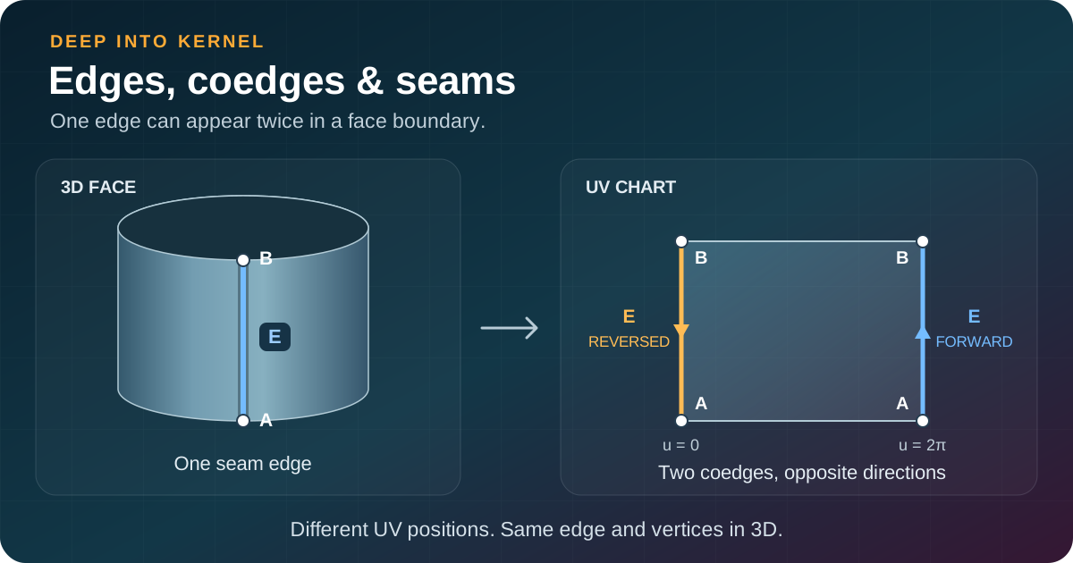
Lines in a CAD viewer can mean different things. They may show free edges, boundaries shared by two faces, or seams used twice by one face. Two lines can coincide in 3D and still represent different edges. One edge can also appear twice in a wire, with two different paths in UV space.
These differences matter in lofts, Boolean operations, offsets, chamfers, fillets, and meshing. A model can look correct in a viewer while boundary data causes a later operation to fail or produce an invalid result.
This Deep into Kernel guide explains how 3D curves, edges, faces, and UV paths work together. Four interactive examples show edge ranges, surface mapping, seams, and parameter matching.
Previous guides explained how OCCT evaluates spline geometry, offsets, and swept surfaces. Here we look at how models use that geometry to define boundaries. A surface tells us where points are. Faces also define which part of that surface belongs to a model.
Geometry, topology, and edge uses
A few terms will help. Geometry describes shape, such as curves and surfaces. Topology describes how vertices, edges, and faces connect. A wire groups edge uses into a boundary. An occurrence means one use of an object; traversal means following those uses in order.
UV space uses two surface coordinates, U and V. A PCurve is a curve in that space. A UV chart shows a chosen part of this space. Tolerance specifies how much deviation is allowed. When a surface repeats after a fixed parameter change, it is periodic.
| Object | Meaning | Coordinates or context |
|---|---|---|
Geom_Curve | Mathematical curve | 3D, parameterized by t |
Geom2d_Curve used as a PCurve | Path in a surface’s parameter space | 2D, (u, v) |
| Curve on surface | Surface evaluated along a PCurve | 3D result, S(p(t)) |
TopoDS_Edge | Reference to edge topology, with position and direction | TShape, location, orientation |
| BRepGraph edge definition | Reusable edge identity | Vertices, tolerance, edge representations |
| BRepGraph coedge | One edge occurrence in a wire | Face context, orientation, PCurve |
A seam is an edge used along both sides of a face boundary. Classic OCCT represents it with TopoDS_Edge; seam status depends on how a face uses it.
For an ordinary shared boundary, two faces share one edge. Each face has its own parameter space and its own boundary PCurve. For a conventional seam, one face uses one edge twice, with opposite boundary directions and two PCurve branches.
Ordinary shared edge                Seam on one face

         Edge E                           Edge E
        /      \                        /      \
    use A      use B                 use A      use B
   Face F1    Face F2                Face F     Face F
   PCurve A   PCurve B               PCurve 0   PCurve 1
To identify a seam, check edge uses within that face. Topological identity matters here: separate edges can coincide in 3D.
Edges use finite curve ranges
Geom_Line continues forever in both directions. Edge bounds can limit its use to a finite range, such as [-1, 1], with vertices at both ends. One curve can support several edge ranges.
Gray shows part of an infinite line. Blue marks a finite edge between Start and End. Drag either handle along this line, or use arrow keys for small changes. A blue point moves within this range. Reversing direction swaps Start and End roles. Stored first and last curve parameters stay unchanged.
TopoDS_Edge inherits three parts from TopoDS_Shape: TShape stores shared topology, location gives its position and rotation, and orientation gives its direction. Edge data is normally stored in BRep_TEdge.
Choose an identity test according to what your application needs to keep:
| Test | Compared properties | Useful for |
|---|---|---|
IsPartner() | TShape | Recognizing shared topology across different placements |
IsSame() | TShape and location | Grouping forward and reversed uses of one placed edge |
IsEqual() | TShape, location, and orientation | Comparing oriented shape references |
Even equal references can occur in different wires or faces. Keep those occurrences separately when following boundaries.
Forward and reversed uses of one edge can pass IsSame() but fail IsEqual(). Reversing a use preserves its stored geometry and parameter limits.
TopoDS_Edge aReversed = TopoDS::Edge(anEdge.Reversed());
bool aSameEdge = anEdge.IsSame(aReversed);   // true
bool aSameUse  = anEdge.IsEqual(aReversed);  // false for FWD versus REV
For an edge count, collect unique placed edges. For a UV boundary, collect wire occurrences with face and orientation. Our cylinder has three unique edges but four occurrences. If your boundary list contains only three entries, check whether a uniqueness filter removed one seam use.
Copying a reference and copying model data
Consider a tool that takes an edge, repairs it, and keeps an original for comparison:
TopoDS_Edge anOriginal = anEdge;
TopoDS_Edge aWorkingEdge = anEdge;
Both variables refer to one TShape. A builder changing stored ranges, tolerance, PCurves, or flags through aWorkingEdge also changes what anOriginal reads. Reversed() creates another oriented reference to that shared data. Changing orientation on a reference is local; editing shared edge data affects all its uses.
This distinction matters for undo, repair previews, and trying several modeling parameters. Keep an independent shape copy when an experiment will modify model data:
#include <BRepBuilderAPI_Copy.hxx>

BRepBuilderAPI_Copy aCopy(aShape, true, false);
TopoDS_Shape aWorkingShape = aCopy.Shape();
Here copyGeom = true copies geometry along with topology. copyMesh = false leaves triangulation out of this geometric working copy. With copyGeom = false, underlying curves and surfaces remain shared, so editing them can still affect the source.
Copy a containing shape in one operation when its internal connections must survive. A box has 12 unique edges shared by six faces. Copying that box preserves 12 shared edges within a new shape. Copying each face separately produces 24 independent edge copies across those faces. Their positions still coincide, but their shared topology has been lost. This is one reason a visually unchanged reconstruction can behave differently in subsequent algorithms.
Edges can carry several representations
An edge may carry a 3D curve, PCurves on supporting surfaces, and polygonal data for display or meshing. These representations serve different uses of one boundary. Geometric curve representations carry parameter ranges and locations; polygonal representations store sampled data.
Curve representations, adaptors, and locations
BRep_TEdge stores tolerance, several flags, and a list of curve representations. A representation is one way to describe edge geometry. Flags record properties such as degeneration and parameter matching. A stored 3D curve is only one possible representation.
| Representation | Data it supplies |
|---|---|
BRep_Curve3D | 3D curve, range, representation location |
BRep_CurveOnSurface | PCurve, surface, range, location |
BRep_CurveOnClosedSurface | Two PCurves on one surface |
| Polygon representations | Sampled boundary points for display or meshes |
BRep_GCurve stores first and last parameters for geometric curve representations. Polygon representations have their own data structures, with parameter arrays where supported.
For example, two edges can use one Geom_Line handle with different ranges. One may use [-1, 1], while another uses [2, 5]. Each edge keeps its own identity and vertices, while its curve representation stores parameter limits.
An edge can obtain its 3D geometry from a PCurve and its supporting surface. BRepAdaptor_Curve lets you evaluate this combination as a 3D curve. Its edge-and-face constructor uses that face’s PCurve. Check curve handles with IsNull() before using them.
Locations also matter. One version of BRep_Tool::Curve() returns a curve and a location. Apply that location before comparing points in model coordinates. The version without a location output can return a transformed copy instead.
PCurve evaluation also requires a consistent placement. UV coordinates belong to a supporting surface’s parameter space. Surface evaluation gives a 3D point; apply its location to obtain model coordinates. Compare both representations in one coordinate system. Otherwise, a placement difference can look like a geometry error. Apply each location once, accounting for transformations already performed by your chosen API.
Choose an evaluator for a specific representation
OCCT offers several ways to evaluate an edge. Their choice determines which stored data you are testing:
| Evaluation path | Data used | Typical use |
|---|---|---|
Geom_Curve::Value(t) | A curve in its own coordinate system | Geometry calculations with separately managed bounds and placement |
BRep_Tool::Curve(edge, location, first, last) | Stored 3D curve, edge range, and combined location | Inspecting or comparing a particular representation |
BRepAdaptor_Curve(edge) | Stored 3D curve, with a curve-on-surface fallback | General 3D evaluation of an edge |
BRepAdaptor_Curve(edge, face) | PCurve on that face, evaluated through its surface | Following a face boundary in 3D |
For example, after editing a PCurve, an edge-only adaptor may still evaluate an unchanged stored 3D curve. It can produce perfectly reasonable points while a face-based calculation follows different geometry. Use the edge-and-face constructor when testing that face representation. For comparison work, explicitly check whether a stored 3D curve exists before comparing both paths.
Adaptors already apply representation placement. Their parameter values still describe stored curve parameterization. To sample a reversed occurrence from Start to End, visit those parameters in descending order.
Vertex positions and curve endpoints
A vertex stores a 3D point and tolerance. An edge also has curve parameters at its endpoints. Evaluating a curve at an endpoint parameter and reading its vertex position are two separate operations, and their coordinates can differ within model tolerances.
When investigating a join, record both. A small difference can reflect an accepted approximation. A larger difference may indicate a wrong parameter, misplaced geometry, or an unsuitable tolerance. Changing a tolerance changes an acceptance condition; it leaves existing coordinates and topological connections in place.
Two independently created vertices can also occupy identical coordinates. A wire builder can connect geometrically coincident endpoints within its tolerance rules, but application code should inspect the resulting wire. Use vertex identity to understand actual connectivity and distances to understand geometric agreement. This helps explain why an imported outline can look closed before its edges form a usable boundary.
A PCurve becomes 3D only through its surface
A PCurve maps a parameter to a point in UV:
p(t) = (u(t), v(t))Surface evaluation maps that UV point into 3D. Include surface location when converting to model coordinates:
Csurface(t) = S(u(t), v(t))A straight line in UV can become a helix on a cylinder. Changing cylinder radius preserves this UV path but changes its physical length and speed.
This matters when choosing sampling steps. On a cylinder of radius 10, a U increment of 0.01 radians covers an arc length of 0.1 model units. At radius 100, it covers 1 unit. Choose boundary sampling from 3D size and deflection requirements; a fixed UV step gives different physical spacing on different surfaces.
A straight UV path becomes a helix
A 2D PCurve evaluated on this cylinder produces a 3D helix. Here U measures angular position and V measures height along its axis.
For this cylinder, let s run from 0 at Start to 1 at End:
p(s) = (2*pi*s, 3s)
S(u,v) = (R cos(u), R sin(u), v)
S(p(s)) = (R cos(2*pi*s), R sin(2*pi*s), 3s)
This straight diagonal in UV makes one full turn around a cylinder and rises by 3 model units. This rise per turn is called pitch. Both ends have matching X and Y coordinates but different Z coordinates, giving this helix distinct endpoints. Switching to a plane preserves this PCurve but produces a straight 3D segment. These results follow from OCCT’s cylindrical surface formula.
This example evaluates UV points on a surface without storing a separate 3D curve. A PCurve can represent a 3D curve on a surface when that curve lies on it within tolerance. Creating a separate 3D curve may require an approximation. This depends on curve type and API choice.
PCurve demo: derivatives and parameter values
A derivative measures how quickly a value changes. Here, Su and Sv describe surface changes in U and V. Applying the chain rule combines these surface derivatives with PCurve derivatives:
Csurface'(t) = Su * u'(t) + Sv * v'(t)This demo calculates these derivatives in C++. Its UV line has speed 1 in its own curve parameter. Slider values run from 0 to 1 across this range. Reported speeds use original curve parameters.
This UV line goes from (0, 0) to (2*pi, 3). Its parameter interval has length L = sqrt((2*pi)^2 + 3^2). For forward traversal, its original parameter is t = L*s. Changing s by 1 therefore changes t by L.
With respect to t, UV speed is 1 and 3D speed is sqrt((2*pi*R)^2 + 3^2) / L. With respect to s, both speeds are multiplied by L. At radius 1, the demo reports 1 for both speeds. This equality follows from our choice of radius and parameterization. Increasing radius keeps UV speed at 1 but increases 3D speed. Here speed means distance per unit of curve parameter.
UV distance is usually different from physical distance. U may be an angle, while V may be a length. Their effect on 3D distance can also change across a surface. On a cylinder of radius R, a change in U gives an arc length of R times that change.
Modeling, surface intersections, import, and repair can all create PCurves. For a plane, BRep_Tool::CurveOnSurface() can create a missing PCurve by projection. This behavior is specific to planar surfaces.
A supporting surface is larger than its face
Geom_Surface tells you how to evaluate (u, v). TopoDS_Face adds a position, orientation, and boundary wires to define a region on that surface. A point can lie on the surface but outside the face.
Consider a flat plate with a circular hole. Its supporting plane extends across both solid material and empty space inside that hole. Outer and inner wires tell these regions apart. A cylinder with an angled cut has a similar issue: its boundary can have a curved outline in UV.
BRepTools::UVBounds() gives a bounding rectangle from available boundary PCurves, falling back to natural surface bounds when that calculation yields an empty box. That rectangle can include points outside the face or inside a hole. A face classifier, such as BRepClass_FaceClassifier, tests point membership. Use coordinates in that face’s UV chart. On periodic surfaces, different UV coordinates can describe one 3D point, so choose a suitable chart.
These examples use simple, filled UV rectangles. Other faces may need more complex outlines. Algorithms working on face boundaries must account for actual loops, including holes and both sides of a seam.
SameRange and SameParameter describe different properties
Two representations can have matching parameter intervals yet produce different points at a given parameter value.
Consider a planar edge with:
C3d(t) = (t, 0, 0)       t in [0, 1]
p(t)   = (t^2, 0)         t in [0, 1]
S(u,v) = (u, v, 0)
Both representations follow one path, share endpoints, and use matching parameter ranges. At t = 0.5, however, the 3D curve gives x = 0.5, while the PCurve composed with the plane gives x = 0.25.
SameRange concerns parameter limits. SameParameter concerns points produced at matching parameter values. In this example, endpoints agree while intermediate points differ.
A closest-point check would report zero distance from either curve to this shared straight segment. A same-parameter check finds a gap of 0.25 at t = 0.5. Use the latter when checking whether a parameter from a 3D curve can also locate its corresponding point on a PCurve. Coincident paths and matching parameterization answer different questions.
The checkbox switches between two prepared cases. A quadratic Bezier PCurve with collinear control points gives the nonlinear case. Each case has matching flags, and our demo compares 101 sample points.
Checking and repairing parameter agreement
BRepLib::SameRange() aligns geometric curve ranges, using a stored 3D curve’s range when available. It processes ranges even if SameRange is already true.
BRepLib::SameParameter() attempts to bring PCurves into parameter agreement with a stored 3D curve. Its edge overload returns immediately when SameParameter is already true, or when a usable 3D curve is missing. For imported data with suspect flags, a shape overload provides forced = true to clear those flags and attempt repair again.
After repair, read SameParameter, compare geometry, and inspect edge and vertex tolerances. The algorithm can modify PCurves and tolerances, and a forced attempt can still leave SameParameter false. Treat the requested tolerance as an input to repair, then check whether the resulting tolerance meets your application’s needs. The demo switches prepared examples rather than running repair operations.
Stored flags record declared model properties. For imported or edited data, verify agreement through geometry evaluation. Sampling illustrates this known formula; checking an arbitrary curve may require more thorough analysis between samples.
Choose tolerances appropriate to each comparison: 3D distance, UV distance, or curve-parameter difference. Each has its own units and meaning.
Compare representations before reusing a split parameter
Suppose an intersection algorithm finds t = 0.5 on a 3D edge. Application code then uses p(0.5) to split that edge’s boundary on a face. In our nonlinear example, those two splits would be placed at x = 0.5 and x = 0.25. Sharing one numeric parameter is useful only when both representations agree at that parameter.
This is why parameter consistency matters beyond drawing. A split must stay consistent with curve ranges, endpoint vertices, and every affected face representation. For a seam, both PCurve branches participate. Let an appropriate topology-building or repair operation update those relationships together.
Our complete C++ diagnostic example reads a stored 3D curve and a face PCurve, reports missing data or incompatible ranges, and measures their separation at 33 matching parameters. It includes translated geometry, both cylinder seam uses, and a shared-data copy example.
| Example | Expected observation |
|---|---|
| Matching planar curves | Zero sampled separation |
Nonlinear PCurve x = t^2 | Maximum sampled separation 0.25 at t = 0.5 |
| Matching edge and face moved together | Zero sampled separation after applying both locations |
| Full-cylinder seam | Two UV branches, each agreeing with its 3D edge within floating-point accuracy |
| Assigned edge reference versus explicit copy | Shared flags for assignment; independent flags for the copy |
Record the parameter of maximum observed separation as well as its distance. That parameter gives a useful place to inspect geometry, continuity, and nearby knots. A sampled maximum is a diagnostic observation; agreement between samples requires further analysis.
How the diagnostic compares points in model coordinates
The example obtains geometry with BRep_Tool::Curve(), Surface(), and CurveOnSurface(). It checks handles, finite ordered ranges, and parameter-limit agreement before sampling. Range comparison uses a parameter tolerance, while point separation is measured in model units.
Its central calculation is:
const gp_Pnt2d aUV = aPCurve->Value(aParameter);
const gp_Pnt aCurvePoint =
  aCurve->Value(aParameter).Transformed(aCurveLocation.Transformation());
const gp_Pnt aSurfacePoint =
  aSurface->Value(aUV.X(), aUV.Y()).Transformed(aSurfaceLocation.Transformation());
const double aGap = aCurvePoint.Distance(aSurfacePoint);
Both points now use one model coordinate system. Using each location exactly once lets a translated or rotated model pass the same comparison as its unplaced geometry.
A result saying that a 3D curve is absent describes a missing comparison path. An edge may still be evaluable through a PCurve and surface. Similarly, different parameter ranges deserve their own report before attempting same-parameter sampling.
For seam inspection, call the function for each oriented edge occurrence obtained from the same face reference. Comparing one branch with its 3D curve answers representation agreement. Comparing adjacent UV endpoints answers boundary connectivity. These are separate measurements, and both can be useful in one report.
The download builds small known examples and checks their expected results. Link it with TKPrim, TKTopAlgo, TKBRep, TKGeomBase, TKG3d, TKG2d, TKMath, and TKernel from one matching OCCT build. In application code, choose sampling density and parameter tolerance for your data, then combine observations with shape validation and operation diagnostics.
Coedges record individual boundary occurrences
Classic TopoDS stores edge uses as oriented occurrences in wires. To get a PCurve, you also need to know which face you are working with.
BRepGraph stores each use as a coedge. Edge definitions hold shared topology and geometry. Coedges record which edge, wire, and face belong to a use. They also record direction and geometry in that face’s UV space.
Edge definition                  Coedge occurrence
  vertices                         parent wire
  tolerance                        referenced edge
  3D curve representation          face context
  3D polygon representation        orientation
                                   PCurve representation
One edge can appear more than once in a wire. In classic TopoDS, direct iteration follows storage order; use BRepTools_WireExplorer for connected traversal. BRepGraph records an ordered coedge sequence. Preserve every repeated use when reading a boundary.
Coedges are similar to half-edges. Topology determines how many uses an edge has: a boundary edge may belong to one face, a shared edge to two faces, and a non-manifold edge to several faces. Seam partners are two uses within the same face.
For forward and reversed boundary uses, reversal swaps start and end roles. Reversing a parent wire changes their combined direction again. Face orientation also affects normal direction. Use OCCT helpers to combine parent and child orientations. Within an assembly, include parent occurrence orientation in this calculation.
Follow each occurrence, then choose its endpoints
Consider edge parameters ranging from 2 to 5. A forward use starts at 2 and ends at 5. A reversed use starts at 5 and ends at 2. Its stored range remains [2, 5]. Endpoint vertices stay attached; only their Start and End roles change.
Seams need an extra step. First choose a PCurve using both oriented edge and face. Then evaluate it along that edge use’s direction. Branch selection and traversal direction are separate steps. Both branches may follow one 3D path but opposite sides of a UV chart.
Face orientation in PCurve queries and normal calculations
Face orientation affects PCurve selection. BRep_Tool::CurveOnSurface(edge, face, ...) handles a reversed face when choosing a seam branch. For work in one face’s UV space, you can use a forward-oriented face reference. Read its wire occurrences and use that same reference for PCurve queries. Keep original face orientation for normal calculations. Use a consistent face orientation for traversal and PCurve queries.
A forward-oriented reference preserves existing geometry and boundaries while providing a consistent orientation for local UV calculations. When following a complete model, combine actual parent and child orientations.
At a regular surface point, cross(Su, Sv) gives a normal direction. Reversing a face flips its normal while preserving surface parameters.
Why a cylinder has two UV sides for one seam
For a cylinder:
S(u,v) = (R cos(u), R sin(u), v)
S(0,v) = S(2*pi,v)
A cylindrical face that covers one full turn can have a rectangular UV boundary. Its left and right sides have different UV coordinates but map to one vertical line in 3D. This line is called a meridian. In a usual BRep model, both sides use one edge.
The full-cylinder example builds one curved face. Its wire has four edge uses but only three different edges: a lower circle, an upper circle, and a seam used twice. Both seam uses pass BRep_Tool::IsClosed(edge, face).
The half-cylinder example builds a curved patch with four different boundary edges. Its surface remains periodic. Each vertical boundary is a separate edge used once by this face. Selecting this option constructs a new half-cylinder patch.
A modeling operation can split a full cylinder into two curved faces with shared vertical edges. Those edges connect different faces. Cylindrical geometry can stay unchanged while face boundaries change.
The UV chart lift control moves displayed U coordinates by a whole number of periods. One cylinder period is 2*pi. Stored PCurves, edge identities, and 3D points stay unchanged.
When following a UV loop, preserve that continuous chart. Reducing each U value independently into [0, 2*pi) sends 2*pi to 0, merging both seam sides in UV. Keep branch coordinates during boundary construction; use whole-period shifts consistently when joining adjacent uses.
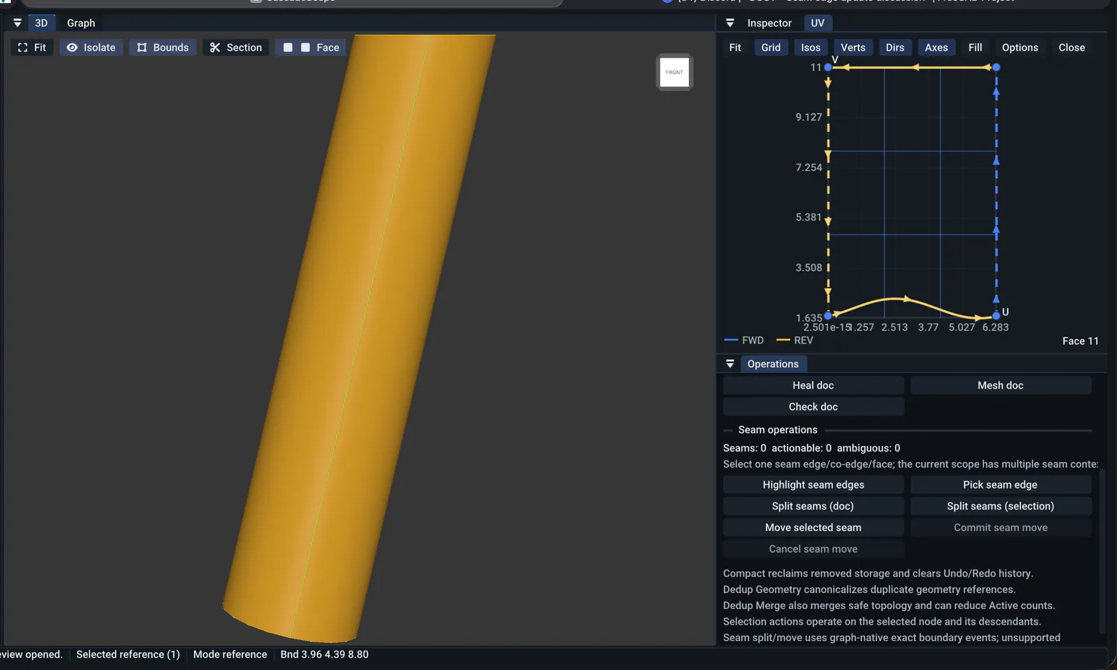
Read 3D boundaries together with their UV charts
The first view shows a selected region with U values from about 0 to 2*pi. Both vertical chart boundaries map to one 3D line on this cylinder.
The second view shows a selected half-cylinder region with U values from about 0 to pi. Surrounding cylindrical geometry is also visible.
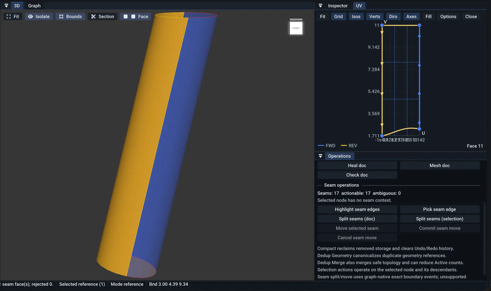
These images show how UV regions follow face boundaries. Use an edge-and-face query to establish seam identity, as in the interactive example. The Operations panel counts apply to its document or selection; the UV panel shows the selected face.
Query a seam in classic OCCT
Use an overload that takes a face:
bool isSeam = BRep_Tool::IsClosed(anEdge, aFace);For geometric BRep data, this checks for a two-PCurve representation associated with that face’s supporting surface and location. The face overload also accepts paired polygons on its triangulation. A true result therefore needs a separate PCurve query before UV work. Endpoint closure is a separate topological property.
BRepTools::IsReallyClosed(edge, face) also checks that an edge appears exactly twice in a face. After import or editing, this helps distinguish stored seam representations from actual boundary uses. Full face validation also requires wire and geometry checks.
C++ example: read both seam occurrences
To keep both seam uses, read every occurrence in the wire:
for (TopoDS_Iterator it(aWire); it.More(); it.Next())
{
  const TopoDS_Edge anOccurrence = TopoDS::Edge(it.Value());
  if (!BRep_Tool::IsClosed(anOccurrence, aFace))
  {
    continue;
  }

  double aFirst = 0.0, aLast = 0.0;
  const auto aPCurve =
    BRep_Tool::CurveOnSurface(anOccurrence, aFace, aFirst, aLast);
  if (aPCurve.IsNull())
  {
    continue;
  }

  const bool isReversed = anOccurrence.Orientation() == TopAbs_REVERSED;
  const gp_Pnt2d aStart = aPCurve->Value(isReversed ? aLast : aFirst);
  // Keep this occurrence together with its face context.
}
Here aWire comes from aFace, with parent location and orientation already included. TopoDS_Iterator composes those with each child by default; applying them again would duplicate that transformation or orientation. It reads children in stored order. Use BRepTools_WireExplorer(wire, face) when you need to follow connected edges. On a broken wire, this explorer may stop before visiting every use. Compare its results with a direct list of wire children when checking a failure. INTERNAL and EXTERNAL uses need separate handling.
On a closed surface, edge-use orientation helps select the PCurve branch. Keep both face and oriented edge use when making this query. Include this context in cache keys so each seam branch remains distinct.
Select a branch for this boundary use, then choose whether to evaluate from first to last parameter or from last to first. A wrong branch can be hard to spot in 3D because both seam branches follow one spatial curve.
Query a seam in BRepGraph
For an existing graph and active edge and face definition IDs, use this face-specific query:
bool isSeam =
  BRepGraph_Tool::Edge::IsSeamOnFace(aGraph, anEdgeId, aFaceId);
If you already have a coedge from traversal, keep it. BRepGraph_Tool::CoEdge::IsSeam() checks for a seam partner. SeamPair() returns that partner’s ID, or an invalid ID if none is found. Use those coedge IDs to query both boundary PCurves, checking that each adaptor contains a usable curve.
C++ example and BRepGraph query details
This example takes a valid, active coedge ID with an owning face. It finds a seam pair and evaluates each branch at its start parameter. Start direction comes from each stored coedge definition:
#include <BRepGraph_Tool.hxx>
#include <array>

bool ReadSeamStarts(const BRepGraph& theGraph,
                   BRepGraph_CoEdgeId theCoEdge,
                   std::array<gp_Pnt2d, 2>& theStarts)
{
  const auto aFace = BRepGraph_Tool::CoEdge::FaceOf(theGraph, theCoEdge);
  const auto aMate = BRepGraph_Tool::CoEdge::SeamPair(theGraph, theCoEdge);
  if (!aFace.IsValid() || !aMate.IsValid())
  {
    return false;
  }

  const std::array<BRepGraph_CoEdgeId, 2> aPair = {theCoEdge, aMate};
  std::array<gp_Pnt2d, 2> aStarts;
  for (std::size_t i = 0; i < aPair.size(); ++i)
  {
    const auto aPCurve =
      BRepGraph_Tool::CoEdge::PCurveAdaptor(theGraph, aPair[i]);
    if (aPCurve.Curve().IsNull())
    {
      return false;
    }
    const bool isReversed =
      BRepGraph_Tool::CoEdge::IsReversed(theGraph, aPair[i]);
    aStarts[i] = aPCurve.Value(isReversed ? aPCurve.LastParameter()
                                        : aPCurve.FirstParameter());
  }
  theStarts = aStarts;
  return true;
}
These APIs are available in the BRepGraph_Tool declarations. Input IDs must be valid and active, and a face owner must be stored. The example reads stored coedge directions. If a parent occurrence is reversed, include that parent direction in your calculation. Reversing a use swaps Start and End roles but keeps its PCurve branch.
These graph queries examine coedge uses. Classic BRep_Tool::IsClosed(edge, face) examines geometric or polygonal representations. In the linked implementation, IsSeamOnFace() looks for uses in one face with different orientations. SeamPair() returns the first other coedge with the same edge and face but a different orientation. For ordinary forward/reversed uses, this finds a seam pair. These are topology queries. Check geometry and count uses separately. On broken data, several partners may be possible; inspect every related coedge. INTERNAL and EXTERNAL uses require separate handling.
For a usual cylinder seam, expect two different coedge IDs with the same edge and face IDs. They have opposite directions and different UV branches. Compare mapped 3D points at corresponding parameters on both branches. With opposite traversal directions, one branch’s Start corresponds to its partner’s End. Uses on two different faces form a shared boundary.
The function returns true when it reads both starts. A false result indicates a missing owning face, seam partner, or usable PCurve. Report these cases separately in a diagnostic tool. Face validity and agreement along both branches require further checks.
Closed, periodic, seam, and degenerated are different
| Property | What to check |
|---|---|
| Closed edge | Endpoint topology; a circle can close on one vertex |
| Periodic surface | Surface parameterization repeats after a period |
| Seam on a geometric face | Two boundary uses with corresponding PCurve branches |
| Degenerated edge | Edge marked as collapsed in 3D |
A flat circular boundary can be closed without being a seam. A half-cylinder face can use a periodic surface without having a seam. At a sphere pole, a whole UV boundary path can map to one 3D point. This degenerated edge is different from the meridian seam.
On a torus, both U and V can be periodic. Moving its UV chart may need whole-period shifts in both directions, (kU, kV).
A degenerated edge is a UV boundary collapsed in 3D
Degenerated edges can be needed in valid faces. A sphere pole is a common example. A whole side of its UV rectangle maps to one 3D point. OCCT keeps that side as an edge with a PCurve to complete its UV boundary. A PCurve and supporting surface normally provide its geometry. Both ends share one pole vertex.
Follow the north-pole boundary
For a sphere centered at the origin with radius R, OCCT uses this surface formula:
S(u,v) = (R cos(v) cos(u), R cos(v) sin(u), R sin(v))

North-pole PCurve: p(t) = (t, pi/2),  t in [0, 2*pi]
Surface image:     S(p(t)) = (0, 0, R)
As t changes, this UV point follows a horizontal path at v = pi/2. Its 3D position stays at the north pole. UV Start (0, pi/2) and End (2*pi, pi/2) are different chart positions. They still refer to one vertex at one 3D point.
A conventional full-sphere chart has four sides with different roles:
| UV side | Image in 3D | Boundary role |
|---|---|---|
| Bottom, v = -pi/2 | South pole | Degenerated edge |
| Right, u = 2*pi | Meridian from south to north | One seam occurrence |
| Top, v = pi/2 | North pole | Degenerated edge |
| Left, u = 0 | Same meridian, traversed back | Other seam occurrence |
Both meridian sides use one seam edge. Top and bottom sides are separate degenerated edges. This wire has four edge uses, three different edges, and two vertices. Other ways of splitting a surface into faces can give different counts.
A degenerated edge joins both seam branches along this upper UV boundary. Keep that path during boundary traversal. Reversal swaps UV Start and End; both still map to one pole.
One vertex locates a pole in 3D. A degenerated edge connects its UV positions, completing a boundary loop for face algorithms.
Checking degenerated edges in imported and generated shapes
Read edge properties, then check geometry
Use BRep_Tool::Degenerated(edge) to read its stored flag. To verify that property, evaluate its geometry. For a flagged edge, get its PCurve on the face. Check that its mapped 3D points stay close to the pole vertex, within that vertex’s tolerance. Missing or incorrect PCurves still need checking. OCCT’s ShapeAnalysis_Wire checks can help find missing pole boundaries and incorrect degenerated edges.
Interpret these properties together with the PCurve and surface:
- Same endpoint vertex: a full circle also starts and ends at one vertex, while its interior points follow the circle.
- Very short 3D length: a small ordinary edge can still represent a real boundary segment. Use its degeneration flag and surface mapping to distinguish these cases.
- Null 3D curve: an ordinary edge can also be represented through a PCurve and surface. Check how the PCurve maps onto the surface.
- Degeneration flag: this records how the edge should behave. Imported data can still contain errors.
A cone tip, called an apex, can have a similar collapsed boundary. A cone patch ending before the tip has an ordinary boundary there. A flat face touching a sphere pole can use an ordinary vertex there. This collapsed UV boundary belongs to a spherical face.
Investigate a problem near a pole
A degenerated edge at a sphere pole or cone tip is expected boundary data. Its zero 3D length alone is a poor reason to remove it during shape cleanup: its PCurve can complete a face’s UV boundary. Before deleting a short edge, check BRep_Tool::Degenerated(edge) and inspect its role on the supporting face.
If a face near a pole displays incorrectly or causes an operation to fail, isolate that face and check it with BRepCheck_Analyzer. Inspect its degenerated edges, their PCurves, and connections to neighboring seam uses. Compare PCurve points mapped through the surface with the pole vertex and its tolerance. These checks help distinguish damaged trimming data from a problem in an operation applied to an otherwise valid face.
A valid face can still show a poor triangulation near a pole. After checking its boundary data, regenerate its triangulation and inspect meshing diagnostics. Changing mesh deflection affects tessellation accuracy; it leaves BRep vertex connections and PCurves unchanged. If those data contain an error, repair the shape before trying the operation again.
Splitting a shared edge: what must stay connected
Suppose two adjacent faces share an edge E, with a 3D curve parameter range [0, 10]. We want to split it at t = 4 while preserving both faces. This small change brings together edge identity, oriented uses, and PCurves: every representation must describe the same two pieces.
Assume E is an ordinary edge with consistent SameRange and SameParameter data. Its PCurves on both faces then use [0, 10], and evaluating them through their surfaces at t = 4 reaches the same 3D point within edge tolerance. The earlier sampling example gives a practical way to investigate that agreement before splitting.
Share the new vertex and both replacement edges
Create one split vertex Vm at C(4) in model coordinates. Two new edges, E0 and E1, connect through that vertex:
Before: V0 ───────────── E [0, 10] ───────────── V1
After:  V0 ── E0 [0, 4] ── Vm ── E1 [4, 10] ── V1
Both pieces can reuse the original supporting curve. Their edge identities, ranges, and vertex connections describe which portions belong to each piece. Reusing a curve handle is useful here: splitting an edge can leave its underlying geometry unchanged.
Use those same two replacement edges in both faces. Creating a separate pair for each face produces coincident boundaries with separate topology. Likewise, two vertices at C(4) can occupy identical coordinates while remaining distinct vertices. Sharing Vm makes the connection explicit.
Suppose one face uses E forward and its neighbor uses it reversed. Connected traversal follows these replacement sequences:
| Original use | Replacement sequence | Vertex path |
|---|---|---|
E forward | E0 forward, E1 forward | V0 → Vm → V1 |
E reversed | E1 reversed, E0 reversed | V1 → Vm → V0 |
Reversal changes both traversal order and each piece’s direction. These sequences describe connected traversal; a wire’s stored child order can differ. Inspect the result with BRepTools_WireExplorer using its face context.
Carry each face’s PCurve onto each piece
For this example, E0 needs the original PCurve on each supporting face restricted to [0, 4]. E1 needs both PCurves restricted to [4, 10]. The split point has one 3D position, while its UV coordinates depend on each face’s surface.
This is where an edge can look correct in a viewer yet cause trouble later. Its 3D curve may show two clean segments while a PCurve still covers [0, 10]. Face algorithms then receive different boundary extents in 3D and UV. Check ranges through each face, including the neighboring face that was outside your initial selection.
For a seam, apply the same reasoning to both PCurve branches on one face. Each replacement edge needs both branches, and both seam occurrences must be replaced in the wire. At the split vertex, those branches can have different UV positions separated by a surface period while mapping to one 3D point. Preserve that separation so the UV boundary still closes around its chart.
What low-level range and flag setters actually change
BRep_Builder::Range(edge, first, last) updates ranges of geometric curve representations by default. Its Only3d option limits the change to the 3D curve; face and surface overloads target a curve-on-surface representation. Choosing an overload controls which stored ranges change.
A range update alone leaves vertex connections and containing wires to be rebuilt. Assigning TopoDS_Edge piece = original also keeps shared edge data, so changing that range affects the original. Create separate edge topology for each piece and deliberately reuse suitable geometry.
BRep_Builder::SameParameter(edge, true) sets a flag. Establish curve agreement before recording it. When representations use different parameterizations, first repair their correspondence or determine a split parameter for each representation. Copying t = 4 into every range works only with the parameter agreement assumed in this example.
After construction, check endpoint parameters, vertex tolerances, PCurve ranges, and both face wires. Validate the assembled shape with BRepCheck_Analyzer; checking each edge in isolation misses connections between pieces and their containing faces. Rebuild affected triangulations and application caches after changing boundaries.
Follow surviving pieces after an operation
A Boolean operation may perform this subdivision for you and keep only some pieces. With history collection enabled, BRepAlgoAPI_BuilderAlgo::Modified(E) reports surviving splits of E in its result. IsDeleted(E) becomes true when both the original edge and all its splits are absent.
This history is useful when a selected edge disappears after a cut. Match its surviving pieces through history, then apply your selection rule: keep every piece, or choose one containing a saved reference point. Recheck each piece’s result-face context before querying its PCurve. A shared supporting curve explains geometric continuity; operation history explains how new edge identities relate to the original selection.
Finding causes of algorithm failures
Lofting, Boolean operations, offsets, chamfers, fillets, and meshing all depend on edge and face data. A shape can look correct in a viewer while errors in connectivity, orientation, or curve representations affect a later algorithm. Problems may appear during construction, intersection, trimming, meshing, or result validation.
Choose a starting point that fits your operation. For a loft, inspect section wires, their directions, and how sections correspond. For a Boolean operation, inspect edges and faces around an intersection. For an offset, chamfer, or fillet, inspect affected faces, selected edges, and their neighbors. Boundary checks help separate input defects from geometric limits such as self-intersections or an unsuitable radius or distance.
A useful first report pairs each symptom with a specific check:
| Observation | Check next |
|---|---|
| 3D endpoints agree, but intermediate points differ at matching parameters | Parameter agreement between curve representations |
| Both seam uses return one UV branch | Oriented edge and face passed to CurveOnSurface(), including cache keys |
| A UV jump is close to one surface period | Branch selection and whole-period shifts |
| Curves agree in local coordinates but differ in model coordinates | Representation locations and transformations applied twice |
| Traversal loses a boundary at a pole | Degenerated edge occurrences and their PCurves |
These observations guide investigation; several errors can produce similar symptoms. Isolate a small set of involved edges, wires, or faces. Record edge occurrences, orientations, parameter ranges, and 3D endpoints. For uses on faces, also record UV endpoints and their mapped 3D positions.
A step-by-step check for edges and face boundaries
- List boundary uses. Keep every wire and edge use with its direction. Compare this with a list of unique edges. Keep repeated seam uses. Check that connected-wire traversal visits every expected use.
- Read geometry in one coordinate system. Check handles, ranges, and locations. Use one consistent face reference for traversal and PCurve queries. Missing 3D curves and missing PCurves need different handling.
- Compare matching points. If both representations exist, evaluate them at the same parameter. Apply their locations before comparing 3D points. Check endpoints and points between them. Interior samples reveal parameter mismatch in our nonlinear example above.
- Follow each boundary. Check vertex connections along wires. For face boundaries, also compare each use’s UV End with the next use’s UV Start. At a periodic seam, keep track of each branch and any whole-period shifts. Applying modulo to each point separately can create a jump in an otherwise connected path.
- Check collapsed boundaries. Pole edges can collapse to a point in 3D but still be needed in UV. Keep these edge uses in the UV loop.
- Check input and output separately. Use
BRepCheck_Analyzertogether with operation-specific diagnostics. A valid input can still encounter geometric limits during an operation. If boundary data needs repair, choose a correction for that defect, rerun the operation, and validate its result. Rebuild affected meshes and cached data after changes.
Check for wrong branches and missing edge uses before increasing tolerance. Use a repair algorithm, then check its resulting flags, geometry, and tolerances. Check what each repair changed, then try the failed operation again.
Useful test shapes include a box, a free wire, a half cylinder, a full cylinder, a sphere with pole edges, and a torus periodic in both directions. Together they cover shared edges, open boundaries, seams, and degenerated edges.
Source reading and related guides
Interactive examples use classic TopoDS and BRep APIs from our demo SDK. They let you compare stored ranges, edge identity, PCurve evaluation, and seam occurrences using OCCT calculations. The C++ examples show how to make similar queries in application code, including BRepGraph coedge traversal.
The BRepGraph example uses a stored owning face ID. Builds with face-context lookup can also find an owning face through parent wires. When adapting this code, check how your API obtains that face context and keep it consistent with boundary traversal.
Use these OCCT declarations and implementations to explore each operation in more detail:
- TopoDS_Shape: identity and orientation
- BRep_Tool: curve, PCurve, seam, and consistency queries
- BRep_Tool implementation: PCurve branch selection and triangulation fallback
- BRepLib: SameRange and SameParameter repair behavior
- BRepTools: UV bounds and IsReallyClosed
- BRepTools_WireExplorer: connection-following traversal and limitations
- BRepGraph_Tool: edge and coedge queries
- BRepBuilderAPI_Copy: topology, geometry, and mesh copying
- BRepAlgoAPI_BuilderAlgo: Boolean operation history
For geometry underlying these representations, continue with B-spline and Bezier Geometry in OCCT and Offset Curves and Swept Surfaces in OCCT. For graph storage and edge uses, see BRepGraph in OCCT 8.0.